What is Feature Engineering?

Feature engineering is a process in which we create new features from the existing features in our data set. The new features are often more relevant to the prediction task than the original set of features, and thus can help the machine learning model achieve better results.

Sometimes the new features are created by applying simple arithmetic operations, such as calculating ratios or sums from the original features. In other cases, more specific domain-knowledge on the data set is required in order to come up with good indicative features.

Feature Engineering Example

To demonstrate feature engineering, we will use the California housing dataset available at Scikit-Learn. The objective in this data set is to predict the median house value of a given district in California, given different features of that district, such as the median income or the average number of rooms per household.

First, we fetch the data set:

from sklearn.datasets import fetch_california_housing

data = fetch_california_housing()
X, y = data.data, data.target
feature_names = data.feature_names

In order to explore the data set, let’s merge the features and the labels into one DataFrame:

mat = np.column_stack((X, y))
df = pd.DataFrame(mat, columns=np.append(feature_names, 'MedianValue'))
df.head()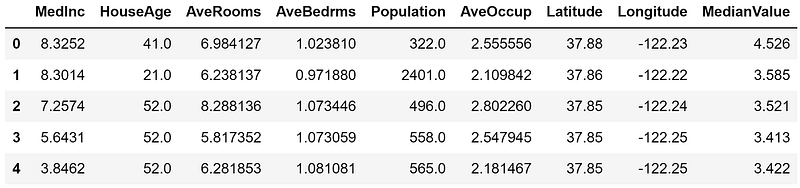

Baseline Model

Before we add any new feature, let’s find out what is the performance of a simple linear regression model on this data set. First, we split our data set into 80% training set and 20% test set:

from sklearn.model_selection import train_test_split

X_train, X_test, y_train, y_test = train_test_split(X, y, test_size=0.2, random_state=0)

Then, we fit a simple LinearRegression model to the training set, and evaluate it on both the training and test sets:

from sklearn.linear_model import LinearRegression

reg = LinearRegression()
reg.fit(X_train, y_train)

train_score = reg.score(X_train, y_train)
print('R2 score on the training set:', np.round(train_score, 5))

test_score = reg.score(X_test, y_test)
print('R2 score on the test set:', np.round(test_score, 5))

The results we get are:

R2 score on the training set: 0.6089
R2 score on the test set: 0.59432

Constructing a New Feature

Now let’s examine our set of features and think if we can come up with new features that might be more indicative to our target (the median house price). For example, let’s consider the feature average number of rooms. The feature by itself may not be so indicative of the house price, since there might be districts that contain larger families with lower income, therefore the median house price will be lower than in districts with smaller families but with much higher income. The same reasoning goes for the feature average number of bedrooms.

Instead of using each of these two features by itself, what about using the ratio between these two features? Surely, houses with a higher ratio of rooms per bedroom imply a more luxury way of living and could be indicative of a higher median house price.

Let’s test our hypothesis. First, we add the new feature to our DateFrame:

df['RoomsPerBedroom'] = df['AveRooms'] / df['AveBedrms']

Now, let’s examine the correlation between our features and the target label (the MedianValue column). To that end, we will use the DataFrame’s corrwith() method, which computes the Pearson correlation coefficient between all the columns and the target column:

df.corrwith(df['MedianValue']).sort_values(ascending=False)

MedianValue         1.000000
MedInc              0.688075
RoomsPerBedrooms    0.383672
AveRooms            0.151948
HouseAge            0.105623
AveOccup           -0.023737
Population         -0.024650
Longitude          -0.045967
AveBedrms          -0.046701
Latitude           -0.144160
dtype: float64

Our new RoomsPerBedroom feature has a much higher correlation with the label than the two original features!

Performance of the Model with the New Feature

Let’s examine how adding the new feature affects the performance of our linear regression model.

We first need to extract the features (X) and labels (y) from the new DataFrame:

X = df.drop(['MedianValue'], axis=1)
y = df['MedianValue']

We also need to split the data set again to training and a test set (note that we are using the same random seed, so the same test set will be used to evaluate the model).

X_train, X_test, y_train, y_test = train_test_split(X, y, test_size=0.2, random_state=0)

Finally, we fit our model and evaluate it:

reg.fit(X_train, y_train)

train_score = reg.score(X_train, y_train)
print('R2 score on the training set:', np.round(train_score, 5))

test_score = reg.score(X_test, y_test)
print('R2 score on the test set:', np.round(test_score, 5))

The results we get are:

R2 score on the training set: 0.61645
R2 score on the test set: 0.60117

The performance has improved on both the training and test sets by just adding this simple feature!

Final Notes

You can find the code examples of this article on my github: https://github.com/roiyeho/medium/tree/main/feature_engineering

Thanks for reading!