What are PCA loadings and how to effectively use Biplots?

A practical guide for getting the most out of Principal Component Analysis.

Image created by the pca library. image by the author.

Principal Component Analysis is the most well-known technique for (big) data analysis. However, interpretation of the variance in the low-dimensional space can remain challenging. Understanding the loadings and interpreting the biplot is a must-know part for anyone who uses PCA. Here I will explain i) how to interpret the loadings for in-depth insights to (visually) explain the variance in your data, ii) how to select the most informative features, iii) how to create insightful plots, and finally how to detect outliers. The theoretical background will be backed by a practical hands-on guide for getting the most out of your data with pca.

If you found this article helpful, use my referral link to continue learning without limits and sign up for a Medium membership. Plus, follow me to stay up-to-date with my latest content!

Introduction

At the end of this blog, you can (visually) explain the variance in your data, select the most informative features, and create insightful plots. We will go through the following topics:

Feature Selection vs. Extraction.
Dimension reduction using PCA.
Explained variance, and the scree plot.
Loadings and the Biplot.
Extracting the most informative features.
Outlier detection.

Gentle introduction to PCA.

The main purpose of PCA is to reduce dimensionality in datasets by minimizing information loss. In general, there are two manners to reduce dimensionality: Feature Selection and Feature Extraction. The latter is used, among others, in PCA where a new set of dimensions or latent variables are constructed based on a (linear) combination of the original features. In the case of feature selection, a subset of features is selected that should be informative for the task ahead. No matter what technique you choose, reducing dimensionality is an important step for several reasons such as reducing complexity, improving run time, determining feature importance, visualizing class information, and last but not least preventing the curse of dimensionality. This means that, for a given sample size, and above a certain number of features the classifier will degrade in performance rather than improve (Figure 1). In most cases, a lower-dimensional space results in more accurate mapping and compensates for the “loss” of information.

In the next section, I will explain how to choose between feature selection and feature extraction techniques because there are reasons to choose between one or another.

Figure 1. The performance of (classifications) models as a function of dimensionality. (image by the author)

Feature selection.

Feature selection is necessary for a number of situations; 1. In case the features are not numeric (e.g., strings). 2. In case you need to extract meaningful features. 3. To keep measurements intact (a transformation would make a linear combination of measurements and the unit to be lost). A disadvantage is that feature selection procedures do require a search strategy and/or objective function to evaluate and select the potential candidates. As an example, it may require a supervised approach with class information to perform a statistical test or a cross-validation approach to select the most informative features. Nevertheless, feature selection can also be done without class information, such as by selecting the top N features on the variance (higher is better).

Feature extraction.

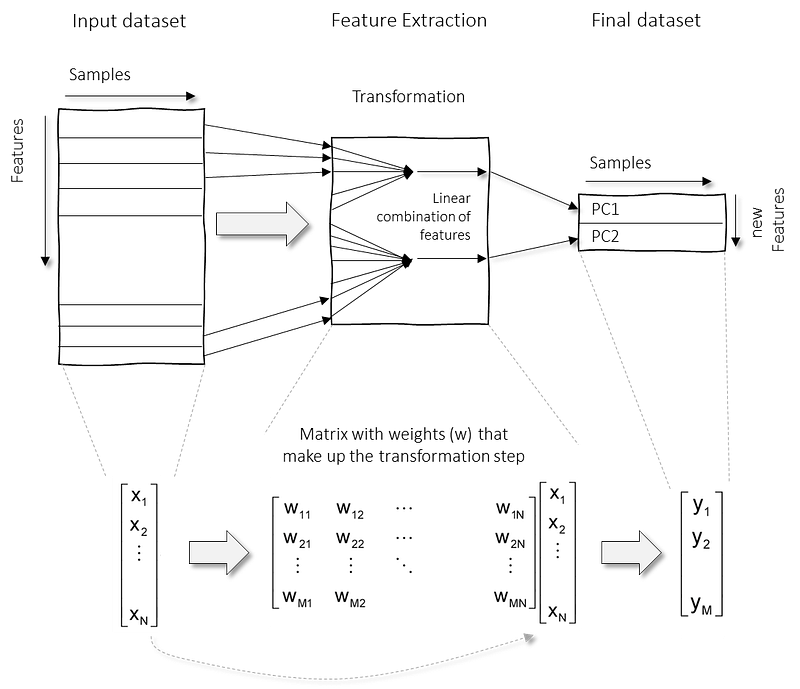
Feature extraction approaches can reduce the number of dimensions and at the same time minimize the loss of information. To do this, we need a transformation function; y=f(x). In the case of PCA, the transformation is limited to a linear function which we can rewrite as a set of weights that make up the transformation step; y=Wx, where W are the weights, x are the input features, and y is the final transformed feature space. See below a schematic overview to demonstrate the transformation step together with the mathematical steps.

A linear transformation with PCA has also some disadvantages. It will make features less interpretable, and sometimes even useless for follow-up in certain use-cases. As an example, if potential cancer-related genes were discovered using a feature extraction technique, it may describe that the gene was partially involved together with other genes. A follow-up in the laboratory would not make sense, e.g., to partially knock out/activate genes.

How are dimensions reduced in PCA?

We can break down PCA into roughly four parts, which I will describe illustratively.

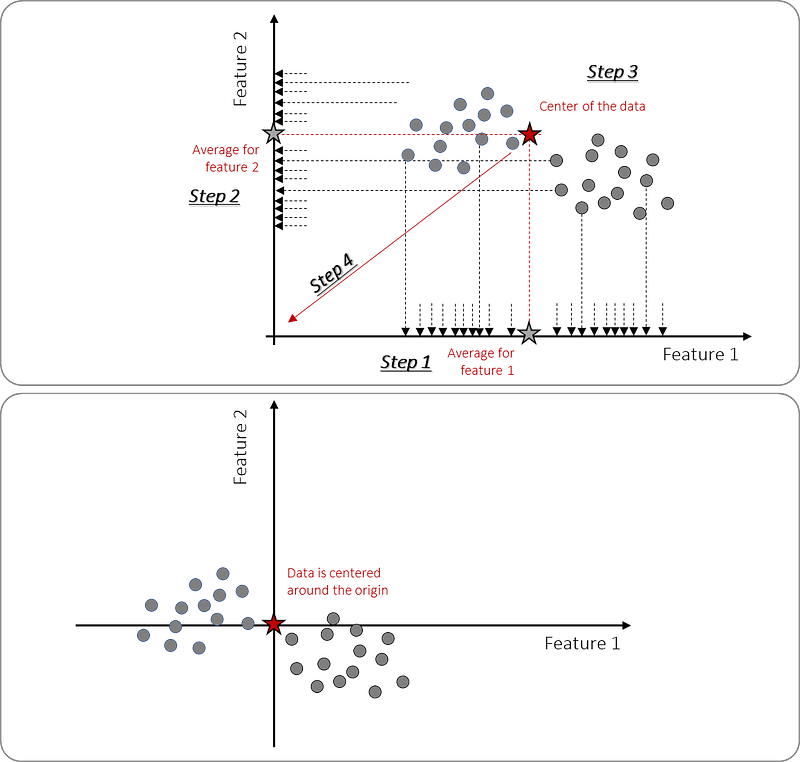
Part 1. Center data around the origin.

The first part is computing the average of the data (illustrated in Figure 4) which can be done in four smaller steps. First by computing the average per feature (1 and 2), and then the center (3). We can now shift the data so that it is centered around the origin(4). Note that this transformation step does not change the relative distance between the points but only centers the data around the origin.

Figure 4: Center data around zero. (image by the author)

Part 2. Fit the line through origin and data points.

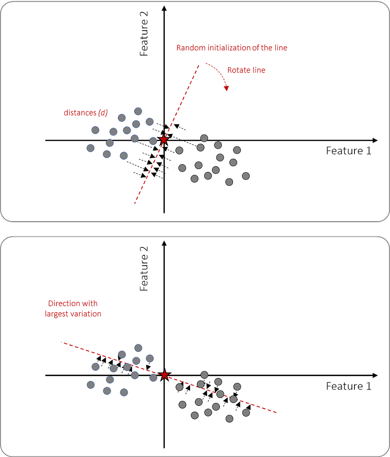
The next part is to fit a line through the origin and the data points (or samples). This can be done by 1. drawing a random line through the origin, 2. projecting the samples on the line orthogonally, and then 3. rotating until the best fit is found by minimizing the distances. However, it is more practical to maximize the distances from the projected data points to the origin which will lead to the same results. The fit is computed using the sum of squared distances (SS) as it will eliminate the orientation of the data points surrounding the line. At this point (Figure 5), we fitted a line in the direction with the maximum variance.

Figure 5: Finding the best fit. Start with a random line (top) and rotate until it fits the data best by minimizing the distances from the data points to the line (bottom). (image by the author)

Part 3. Computing the Principal Components and the loadings.

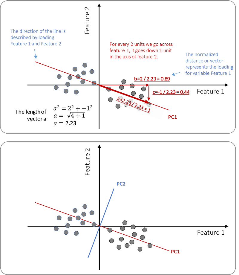
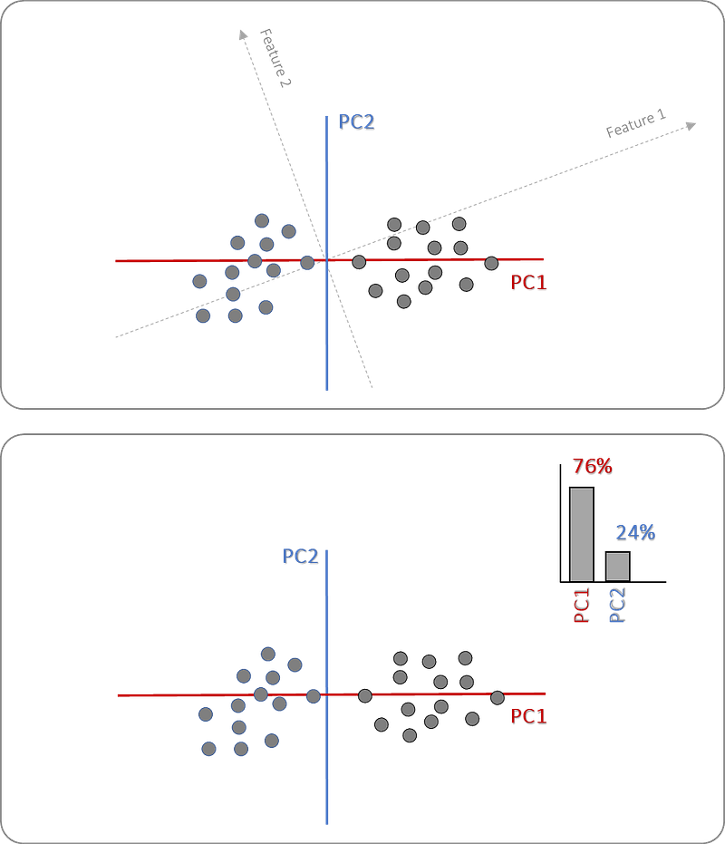
We determined the best-fitted line in the direction with maximum variation which is now the 1st Principal Component or PC1. The next step is to compute the slope of PC1 that describes the contribution of each feature for PC1. In this example, we can visually observe that data points are spread out more across feature 1 than feature 2 (Figure 6). The slope of the red line is representative of our visual observation; for every 2 units we go across feature 1 (to the right), it goes down 1 unit in the axis of feature 2. Or in other words, to make PC1 (the red line), we need 2 parts of feature 1 and -1 part of feature 2. We can describe these “parts” as vectors b and c which we can then use to compute vector a. Vector a will get the value of 2.23 (see figure 6). This is what we call the eigenvector for this particular PC.

However, we need to standardize toward the so-called “unit vector” which we get by dividing all vectors by a=2.23. Thus vector b=2/2.23=0.85, vector c=1/2.23=0.44 and vector a=1 (aka the unit vector). Thus, in other words, the range of these vectors is between -1 and 1. If for example vector b would have been very large, such as a value towards 1, it would mean that feature 1 contributes almost entirely to PC1.

The next step is to determine PC2 which is a line that goes through the origin and is also perpendicular to the first PC. In this example, there are only two features but if there were many more features, the third PC would become the best fitting line through the origin and perpendicular to PC1 and PC2. As described before: New latent variables, aka the PCs, are a linear combination of the initial features. The proportion of each feature that is used in the PC is named the coefficient.

Loadings

It is important to realize that the principal components are less interpretable and don’t have any real meaning since they are constructed as linear combinations of the initial variables. But we can analyze the loadings which describe the importance of the independent variables. The loadings are from a numerical point of view, equal to the coefficients of the variables, and provide information about which variables give the largest contribution to the components.

Loadings range from -1 to 1.
A high absolute value (towards 1 or -1) describes that the variable strongly influences the component. Values close to 0 indicate that the variable has a weak influence on the component.
The sign of a loading (+ or -) indicates whether a variable and a principal component are positively or negatively correlated.

Part 4. The transformation and explained variance.

We computed the PCs and we can now rotate (or transform) the entire dataset in such a manner that the x-axis is the direction where the largest variance is seen (aka PC1). Note that the transformation step will cause the values of the original feature will be lost. Instead, each PC will contain a proportion of the total variation but with the explained variance we can describe how much variance each PC contains. To compute the explained variance we can divide the sum of squared distances (SS) for each PC by the number of data points minus one.

Figure 7. Transformation of the entire dataset and determining computing the explained variance. (image by the author).

Part 0. Standardization

Before we do parts 1 to 4, it is crucial to get the data in the right shape by standardization and this should therefore be the very first part. Because we search for the direction with the largest variance, a PCA is very sensitive to variables that have different value ranges or to the presence of outliers. If there are large differences between the ranges of initial variables, the variables with larger ranges will dominate over those with small ranges. I will demonstrate this in the next section. To prevent this, we need to standardize the range of the initial variables so that each variable contributes equally to the analysis. We can do this by subtracting the mean and dividing it by the standard deviation for each value of each variable. Standardization involves rescaling the features such that they have the properties of a standard normal distribution with a mean of zero and a standard deviation of one. This is also named a z-score standardization for which Scikit-learn has the StandardScaler(). Once the standardization is done, all the variables should be on the same scale.

The PCA library.

A few words about the pca library that is used for the upcoming analysis. The pca library is designed to tackle a few challenges such as:

Analyze different types of data. Besides the regular PCA, the library also includes sparse PCA for which the sparseness is controllable by the coefficient of the L1 penalty. And there is a truncated SVD that can efficiently handle sparse matrices as it does not center the data before computing the singular value decomposition.
Computing and plotting the explained variance. After fitting the data, the explained variance can be plotted: the scree plot.
Extraction of the best-performing features. The best-performing features are returned by the model.
Insights into the loadings with the Biplot. To retrieve more insights of the variation of the features and separability of the classes in relation to the PCs.
Outlier Detection. Outliers can be detected using two well-known methods: Hotelling-T2, and SPE-Dmodx.
Removal of unwanted (technical) bias. Data can be normalized in such a manner that the (technical) bias is removed from the original data set.

What benefits does pca offer over other implementations?

At the core of the PCA library, the sklearn library is used to maximize compatibility and its integration in pipelines.
Standardization is built-in functionality.
Contains the most-wanted output and plots.
Simple and intuitive.
Open-source.
Documentation page with many examples.

A practical example to understand the loadings.

Let’s start with a simple and intuitive example to demonstrate the loadings, the explained variance, and the extraction of the most important features.

First, we need to install the pca library.

pip install pca

Creating a Synthetic Dataset.

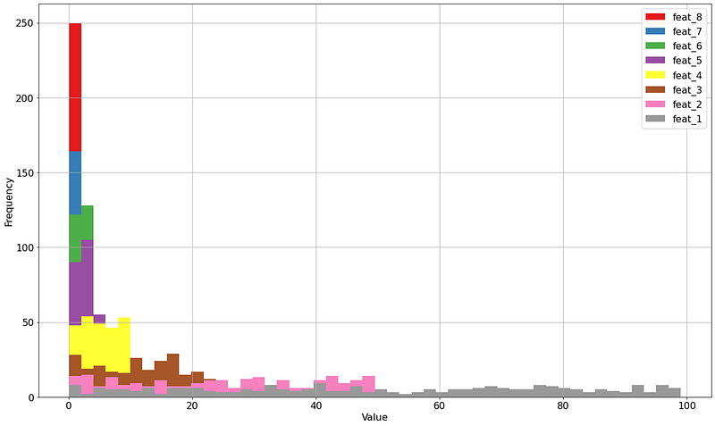
For demonstration purposes, I will create a synthetic dataset containing 8 features and 250 samples. Each feature will contain random integers but with increasing variance. All features are independent of each other. Feature 1 will contain integers in the range [0, 100] (and thus the largest variance), feature 2 will contain integers in the range of [0, 50], feature 3 with integers in the range [0, 25], and so on (see code block below). For the sake of example, I will not normalize the data to demonstrate the principles. This dataset is now ideal to 1. demonstrate the principles of PCA, 2. demonstrate the loadings and the explained variance, and 3. the importance of standardization (or the lack of it). Before we continue I want to repeat again: when working with real-world datasets, it is advised to carefully look at your data and normalize accordingly to bring each feature to the same scale.

If we plot the histogram of the 8 features, we can see that feature 1 (grey) has the largest variance, followed by pink (feature 2), and then brow (feature 3), etc. The smallest variance is seen in the red bar (feature 8).

Figure 8. Histogram of the 8 independent features (image by the author).

What should we expect to find?

Before we do the PCA analysis on this controlled example dataset, let’s think through what we should expect to find. First of all, with the PCA analysis, we aim to transform the space in such a manner that features with the largest variance will be shown in the first component. In this dataset, we readily know which features contain the largest variance. We expect the following:

The rotation of the high-dimensional space will be in such a manner that feature 1 will be the main contributor in the first Principal Component (PC1).
According to the PCA methodology, the second Principal Component (PC2) should be perpendicular to PC1, move through the origin, and in the direction with the second-largest variance. The largest contribution will be by feature 2.
The third Principal Component (PC3) should be perpendicular to PC1 and PC2 and in the direction with the third-largest variance. In our example, we know that feature 3 will be the main contributor.

To summarize, we expect to see Features 1, 2, and 3 back as the major contributors for PC1, PC2, and PC3 respectively. We should be able to confirm our expectations by using the loadings and the biplot.

How do we visualize the loadings?

Loadings are visualized by arrows that are under an angle and have a certain length. The angle represents the contribution of a particular feature in the direction of the PCs where it contributes. The length of the arrow depicts the strength of the contribution of the feature in that direction. In a 2D plot, a (near) horizontal arrow (along the x-axis) describes that the feature contributes toward PC1. On the other hand, a vertical arrow describes that a feature contributes the most to the y-axis, and towards PC2. An arrow under a certain angle describes that the particular feature contributes to various PCs in that direction. The length of the arrow depicts the strength or load of the feature in the particular PC. In our example, we expect that feature 1 contributes the most for PC1, and will be almost horizontal and thus will get a value near absolute 1. Feature 2 contributes most to PC2 and will be almost vertical, and will have a value near absolute 1. Feature 3 contributes most to PC3 and will be in the direction of the z-axis., and get a value of near-absolute 1.

The PCA results.

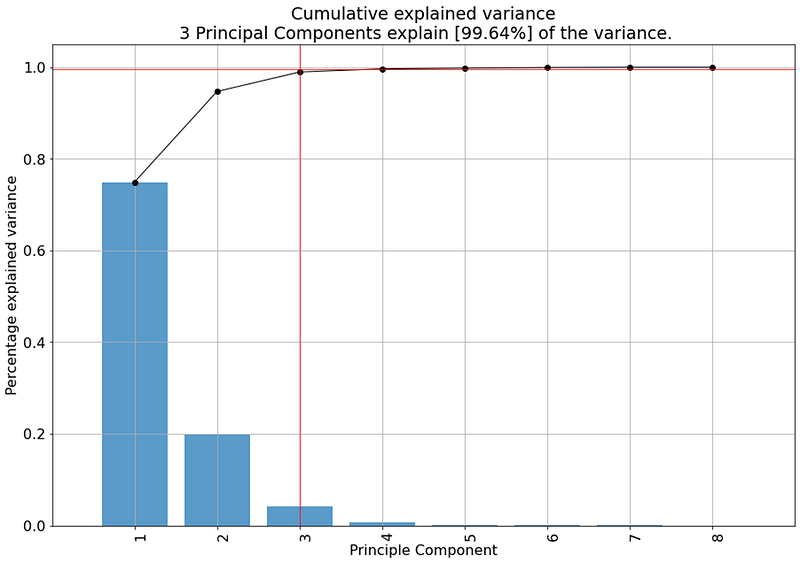
We theorized about what we should expect, and now we can compute the Principal Components with their loadings and the explained variance. For this example, I will initialize pca with n_components=None and thereby not remove any of the PCs. Note that the default is: n_components=0.95 which depicts that the reduction of PCs is up to 95% of the explained variance.

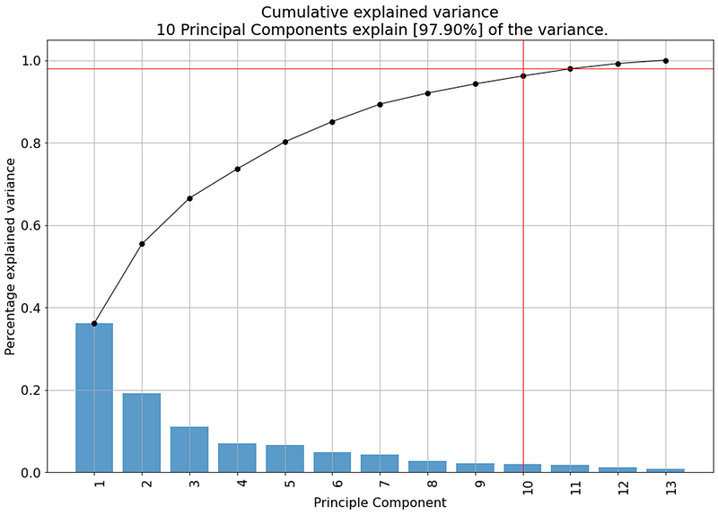
After we fit and transform the data, we can start investigating the features and the variation in the data. First, we can examine the explained (cumulative) variance with the so-called scree plot (Figure 9). We can see that PC1 and PC2 cover over 95% of the variation, and the top 3 PCs cover 99.64% of the total variation. The default setting in the pca library is that only the PCs are kept up to 95% explained variance (thus the top 3 in this case). Note: If the scree plot would result in bars that are equally high, then the top n PCs would not create a very accurate representation of the data. This would have happened if we would have normalized the data at the start (we are working with random data).

Figure 9. Scree plot with the (cumulative) explained variance (image by author).

The 2-dimensional plot with the samples is depicted in Figure 10. Here we see that the samples are uniformly distributed. Note that the values range heavily between the x-axis and y-axis.

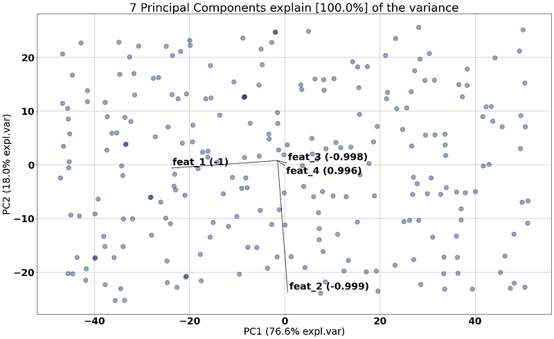
Figure 10. Two-dimensional plot of the random data with PC1 and PC2. We can remove the legend, and set a maximum number of loadings. (image by the author).

Let’s focus on only the loadings and remove the scatter from the plot (Figure 11, by setting the parameter cmap=None). We can clearly see that the largest contributor for the first principal component is feature 1 as the arrow is almost horizontal and has a loading of almost -1 (-0.99). We see similar behavior for feature 2 with PC2, and for feature 3 with PC3 but for PC3 we need to make a 3D plot to see the top 3 features.

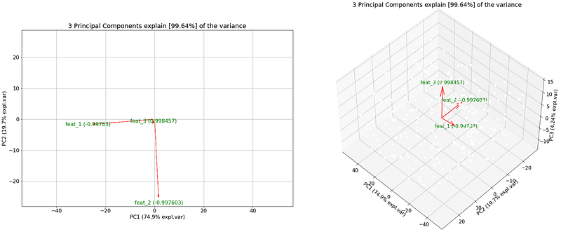
Figure 11. Two and Three-dimensional plots with the loadings. (image by the author).

Note that all these results are also stored in the output of the model as shown in the code block above. At this point, we can now interpret the loadings with the arrows, the angle, the length, and the associated features. You should realize that we used random integers and still find potential “interesting” contributors to the PCs. Without normalization, the feature with the largest range will have the largest variance and be the most important feature. With normalization, all features would have more or less similar contributions in the case of random data. Always be thoughtful when analyzing your data.

In the next section, we will analyze a real data set and see how the loadings behave and can be interpreted.

Wine dataset.

So far we have used a synthetic dataset to understand how the loadings behave in a controlled data set. In this section, we will analyze a more realistic data set and describe the behavior and contribution of features across the high-dimensional space. We will import the wine dataset and create a data frame that contains 178 samples, with 13 features and 3 wine classes.

The range of the features heavily differs and a normalization step is therefore important. The normalization step is a build-in functionality in the pca library that can easily be set by normalize=True. For demonstration purposes, I will set n_components=None to keep all PCs in the model.

After the fit and transform we can output the top-performing features that are stored in the key “topfeat”. Here we see which variables contribute most to which PCs. With the scree plot, we can examine the variance that is captured across the PCs. In Figure 12 we can see that PC1 and PC2 together cover almost 60% of the variation in the dataset. That's quite OK! We also see that we need 10 PCs to capture >95% of the variation.

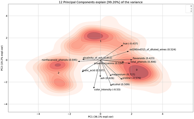
Figure 12. Scree plot wine dataset (image by the author).

If we make the biplot and color the three classes, we can directly notice that the first 2 PCs separate the 3 classes quite well. The first PC captures 36.1% of the variation and the second PC 19.2%. The loadings will now help us to deeper examine how the variables contribute to the PCs, and how classes are separated. The feature that most contribute to the x-axis, and thus for PC1 is flavonoids, whereas, for PC2 (the y-axis), the largest contributor is from the variable color_intensity. The features with a wider angle, such as hue and malic_acid contribute partly to PC1 and PC2.

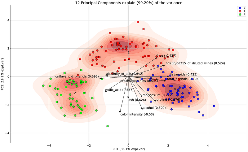
Figure 13. Biplot of the wine dataset. Samples are colored on class information. (image by the author).

Let’s start deeper investigating the flavanoids variable that contributes to PC1. The angle of the flavanoid’s arrow is positive, almost horizontal, and has a score of 0.422. This suggests that some of the variances in the x-axis should come from the flavonoids variable. Or in other words, if we would color the samples using the flavanoids values, we should expect to find samples with low values on the left side and high values on the right side. We can easily investigate this as follows:

model.biplot(labels=df['flavanoids'].values, legend=False, cmap='seismic')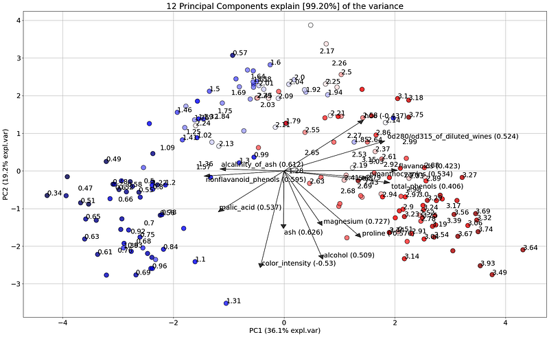

Figure 14. Biplot of the wine dataset. Samples are colored on *flavonoids values* (image by the author).

And indeed, it is nice to see that the samples are colored blue-ish (low value) on the left side and red-ish (high value) on the right side. The loading thus accurately described which feature contributed the most along the x-axis, and the value range.

Positive loadings indicate that a variable and a principal component are positively correlated whereas negative loadings indicate a negative correlation. When loadings are large, (+ or -) it indicates that a variable has a strong effect on that principal component.

Let’s take another one. The best contributor for PC2 is color_intensity. This arrow is downwards and we should expect that the values are thus negatively correlated with PC2. Or in other words, samples with high values for color_intensity are expected at the bottom and low values at the top. If we now color the samples using the color_intensity (Figure 15), it is clear that the variation is indeed along the y-axis.

# 2D plot with samples colored on color_intensity
model.biplot(labels=df['color_intensity'].values, legend=False, cmap='seismic')

# 3D plot with samples colored on color_intensity
model.biplot3d(labels=df['color_intensity'].values, legend=False, label=False, cmap='seismic')

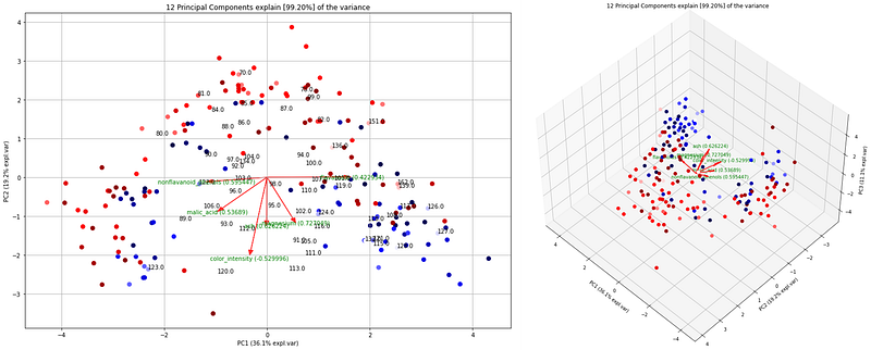
# 2D plot with samples colored on magnesium
model.biplot(labels=df['magnesium'].values, legend=False, cmap='seismic')

# 3D plot with samples colored on magnesium
model.biplot3d(labels=df['magnesium'].values, legend=False, label=False, cmap='seismic')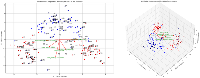

Figure 14. Biplot of the wine dataset. Samples are colored on color_intensity values (image by author).

Let’s also have a look at the magnesium loading. The loading for this variable has a wider angle and is downwards directed which means that it contributes partly to PC1 and PC2. Creating the 3D plot and coloring the samples on the magnesium values makes it clear that some of the variations are also captured along PC3.

Figure 14. Biplot of the wine dataset. Samples are colored on magnesium values (image by the author).

Besides coloring the samples, it is also possible to further investigate the samples across other dimensions such as 4th, 5th, etc PCs with their loadings. With these analyses, we gained much intuition in the variation of the variables and we can even hypothesize how the classes are separated. All these insights are an excellent starting point to discuss the possible follow-up steps and to set some expectations.

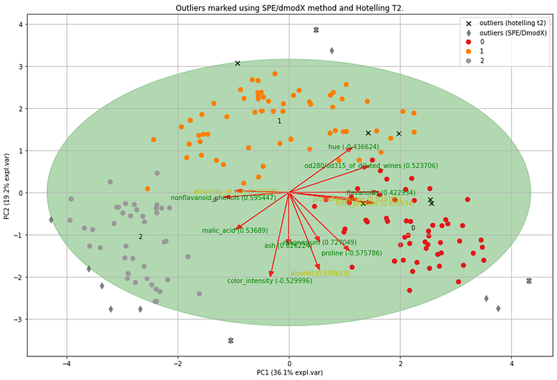
Outlier detection.

The pca library contains two methods to detect outliers: Hotelling’s T2 and SPE/DmodX. Hotelling’s T2 works by computing the chi-square tests whereas the SPE/DmodX method is based on the mean and covariance of the first 2 PCs. Both methods are complementary to each other in their approach, and computing the overlap can therefore point toward the most deviant observations. When we analyze the wine data set, we detected three overlapping outliers overlap between the methods. If you need to investigate the outliers, those will be an excellent start. Alternatively, outliers can be ranked y_proba (lower is better) for Hotelling T2, and y_score_spe for the SPE/DmodX method (larger is better).

Figure 15. Outliers detected using the SPE/DmodX method are depicted with diamonds. Outliers detected using the Hotelling T2 method are depicted with crosses. (image by the author)

Wrapping up.

Each PC is a linear vector that contains proportions of the contribution of the original features. The interpretation of the contribution of each variable to the principal components can be retrieved using the loadings and visualized with the biplot. Such analysis will give intuition about the variation of the variables and the class separability. This will help to form a good understanding and can provide an excellent starting point to discuss the follow-up steps. As an example, you can question whether it is required to use advanced machine learning techniques for the prediction of a specific class or whether we can set a single threshold on a specific variable to make class predictions.

Furthermore, the pca library provides functionalities to remove outliers using the Hotelling T2 test and SPE/Dmodx method. I did not go into the removal of unwanted (technical) variance (or bias) but this can be done using a normalization strategy.

This is it. Let me know if something is not clear or if you have suggestions to further improve the pca library!

Be safe. Stay frosty.

Cheers, E.