Weisfeiler Leman Graph Isomorphism with Molecular Graphs

Graph Neural Networks (GNNs) represent a significant advancement in neural network architectures, specifically tailored to learn vector representations of nodes and entire graphs within a supervised, end-to-end learning framework. However, after careful studies from several authors it has been shown that capabilities of GNNs are in relation to the one-dimensional Weisfeiler-Leman (1-WL) graph isomorphism heuristic. GNNs exhibit an expressive power equivalent to that of the 1-WL heuristic in discerning non-isomorphic subgraphs.

Before diving deep first lets understand what is Graph Isomorphism

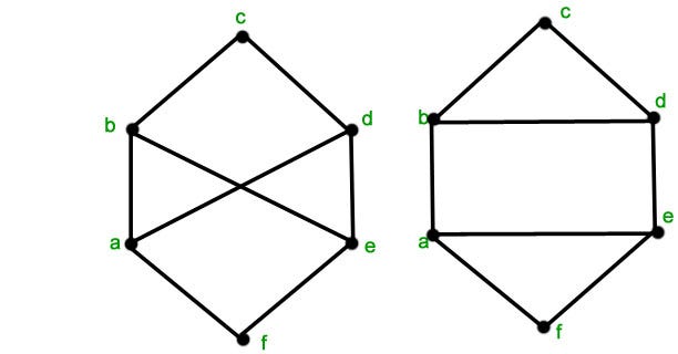
Two graphs G and G’ are isomorphic if there exists a matching between their vertices so that two vertices are connected by an edge in G if and only if corresponding vertices are connected by an edge in G’. The graph isomorphism problem asks whether two graphs are topologically identical. This is a challenging problem: no polynomial-time algorithm is known for it yet been. The following diagram makes it much more simple — both these graphs are isomorphic.

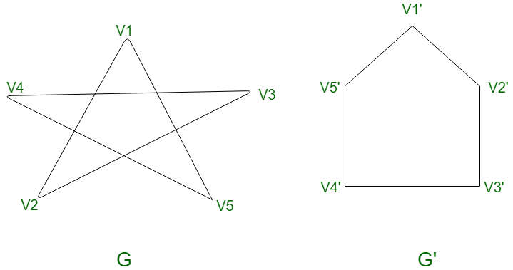
What about this ?

Non — Isomorphic Taken from Geeks For Geeks

The second graph has a circuit of length 3 and the minimum length of any circuit in the first graph is 4. Hence the given graphs are not isomorphic.

Weisfeiler-Lehman (WL) graph isomorphism test was originally proposed by Boris Weisfeiler and Andrei Lehman in the 1960s as an algorithm to test graph isomorphism(graphs which have same structure: identical connections but nodes are a permutated) — whether two graphs are structurally identical. The WL test can tell if two graphs are non-isomorphic, but it cannot guarantee that they are isomorphic. Researchers in graph learning noticed that this test and the way GNNs learn are oddly similar. In the WL test, It iteratively updates the labels of graph nodes (atoms in molecules) based on their own labels and the labels of their neighbors.

The way it works is :

Let G=(V,E) be a graph with vertex set V and edge set E. Each Vertex v ∈ V is assigned an initial label l(0) (v). At each iteration k, update the label of each vertex based on its own label and the set of labels of its adjacent vertices.

Where N(v) denotes the neighbors of vertex v, and HASH is a function that uniquely encodes the combined label

They adapted this idea into the WL sub-tree kernel, which uses the same iterative relabeling process. They define the kernel between two graphs based on the similarity of their node label distributions after several iterations of relabeling. For two graphs G and H, the WL sub-tree kernel after T iterations is given as:

Let, p(G) be a feature vector where each element counts the occurrences of a specific label in G after T. The WL kernel is then the dot product of these feature vectors:

K(G,H) = (p(G),p(H))

This counts the number of label patterns the two graphs have in common.

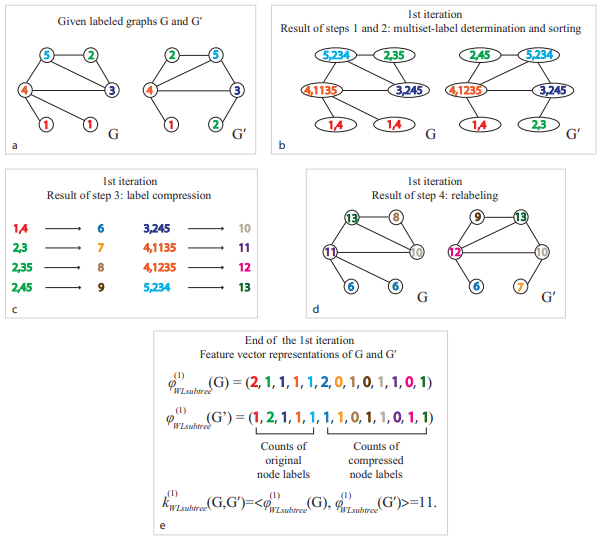
I illustrate the key steps from the above figure below,

The original node labels are used to create multiset labels for each node. These labels are based on the sorted set of labels of neighboring nodes.
Label compression : The multiset labels are then compressed into new labels using a function that maps each unique string of labels to a unique identifier. This step is crucial for capturing the local topology of the graph around each node.
Relabeling : The nodes of the graphs are relabeled with these new compressed labels. This relabeling process effectively encodes the neighborhood structure of each node into a single label.
Feature vector representation (End of the 1st iteration): After the relabeling step, each graph is represented by a feature vector. This vector counts the occurrences of both the original and the compressed node labels in the graph. The feature vectors of G and G’ are then used to compute the kernel value, which quantifies the similarity between the two graphs based on their common labels.

Many GNN architectures, especially those following the message passing framework, bear a conceptual resemblance to the WL algorithm. In each layer, a node’s representation is updated based on its own and its neighbors’ representations.Both GNNs and the WL sub-tree kernel iteratively aggregate neighbor information to encode the graph structure. This aggregation is akin to capturing the local neighborhood of each node, allowing the methods to distinguish different graph topologies.

Now using WL sub-tree kernel we will show how to compute molecular similarity. Keep in mind I am not using any kind of atomic features or edge features into account which can make it more intuitive. First i define some functions which would be required to compute WL based similarity on molecular graphs. I used rdkit to read molecules and networkx to convert them into graph into smiles_to_nx().

import networkx as nx
from rdkit import Chem
import numpy as np
from collections import Counter

def smiles_to_nx(smiles):
    mol = Chem.MolFromSmiles(smiles)
    G = nx.Graph()
    for atom in mol.GetAtoms():
        G.add_node(atom.GetIdx(), label=atom.GetSymbol())
    for bond in mol.GetBonds():
        G.add_edge(bond.GetBeginAtomIdx(), bond.GetEndAtomIdx())
    return G

def weisfeiler_lehman_step(G):
    new_labels = {}
    for node in G.nodes():
        neighbors_labels = [G.nodes[neighbor]['label'] for neighbor in G.neighbors(node)]
        new_label = hash((G.nodes[node]['label'], tuple(sorted(neighbors_labels))))
        new_labels[node] = new_label
    nx.set_node_attributes(G, new_labels, 'label')

def weisfeiler_lehman_hash(G, n_iter=5):
    for _ in range(n_iter):
        weisfeiler_lehman_step(G)
    return Counter([G.nodes[node]['label'] for node in G.nodes()])

def wl_kernel_normalized(graphs, n_iter=5):
    wl_hashes = [weisfeiler_lehman_hash(G, n_iter) for G in graphs]
    n = len(graphs)
    kernel_matrix = np.zeros((n, n))
    normalized_matrix = np.zeros_like(kernel_matrix)

    for i in range(n):
        for j in range(n):
            kernel_matrix[i, j] = sum((wl_hashes[i] & wl_hashes[j]).values())

    # Normalize the kernel matrix
    for i in range(n):
        for j in range(n):
            norm_factor = np.sqrt(kernel_matrix[i, i] * kernel_matrix[j, j])
            normalized_matrix[i, j] = kernel_matrix[i, j] / norm_factor if norm_factor != 0 else 0
    return normalized_matrix

The functions :

weisfeiler_lehman_step() : It result in a graph where each node has a new label that reflects not just its own original label but also the structure of its immediate neighborhood.

For each node in the graph, the function aggregates (collects and combines) the labels of the node’s immediate neighbors.
It then generates a new label for the node by combining its current label with this aggregated neighbor information.
This new label typically involves a hashing process to ensure uniqueness and manage the label’s complexity.

weisfeiler_lehman_hash() : This function computes a hash (a unique identifier) for an entire graph based on the labels of its nodes, particularly after applying several iterations as the user input of the Weisfeiler-Lehman step. These labels are combined (for instance, by creating a sorted tuple) and hashed to produce a single hash value representing the entire graph.

wl_kernel_normalized(): This function calculates a normalized kernel matrix based on the Weisfeiler-Lehman hash values for a set of graphs. After computing weisfeiler-lehman hash for each graph into the kernel matrix ,it’s normalized so that the diagonal elements (representing a graph’s similarity with itself) are 1, and off-diagonal elements scaled to represent relative similarities.

Below is the function to calculate the matrix, I include one very similar structure how it calculates for a single atom.

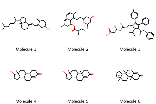
smiles_list = [
    "CC(C)CCCC(C)C1CCC2C1(CCCC2=CC=C3CC(CCC3=C)O)C",
    "CCC(C)C(=O)OC1CC(C=C2C1C(C(C=C2)C)CCC3CC(CC(=O)O3)O)C",
    "CC(C)C1=C(C(=C(N1CCC(CC(CC(=O)O)O)O)C2=CC=C(C=C2)F)C3=CC=CC=C3)C(=O)NC4=CC=CC=C4",
    "CC12CCC3C(C1CCC2O)CCC4=CC(=O)CCC34C",
    "CC12CCC3C(C1CCC2O)CCC4=CC(=O)CCC34C","O=C4CC[C@@]3([C@@H]1[C@H]([C@H]2[C@](CC1)(CCC2)C)CCC3=C4)C"]

graphs = [smiles_to_nx(smiles) for smiles in smiles_list]
km_norm = wl_kernel_normalized(graphs, n_iter=2)
## Print the matrix 
print(km_norm)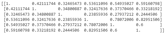

Similarity Matrix of molecules when niter=2 .

When you increase the iterations to 4,5,6 the matrix changes to

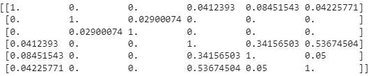
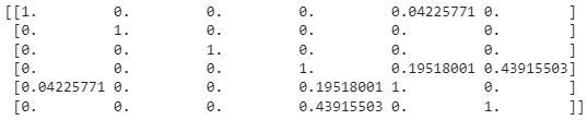
In the early iterations, node labels predominantly reflect immediate or close neighborhood structures, leading to more commonality between different graphs. This commonality results in higher similarity scores in the kernel matrix. As the number of iterations increases, the labels starts to reflect wider neighborhoods. The increased specificity and uniqueness of these labels mean that it’s less likely for different graphs to share the same (or similar) labels, especially if the graphs have diverse structures. The matrix entries represent more specific and less commonly shared structural features between the graphs.

One can include atomic properties in the labels, each iteration of the WL algorithm captures more than just the topological structure; it also captures the chemical environment surrounding each atom. This can lead to a more chemically meaningful representation of the molecular graph, as the updated labels reflect both the connectivity and the chemical context of the atoms.

There is an excellent blog post by David Bieber and this article by Michael Bronstein which give be ideas to write this blog.

If you enjoyed reading this, and/or want to be kept in the loop about the next blog, follow me on Medium.

Feel free to connect with me on LinkedIn and tell me if you end up using this code in your research/job.