Visualizing the Electric Field of a Dipole in Python

Your Daily Dose of Scientific Python

In this article, we’ll discuss how to visualize the electric field of a dipole using Python and the Matplotlib library. We’ll also provide some background on electric dipoles and the equations used to calculate their electric field.

Background

An electric dipole consists of two equal and opposite point charges separated by a distance d. These charges create an electric field that can be calculated using Coulomb’s law. If we place the dipole in a uniform electric field, the dipole will experience a torque that tends to align the dipole moment vector with the electric field.

The electric field of an electric dipole can be expressed using the following equation (ignoring constants like the vacuum permittivity:

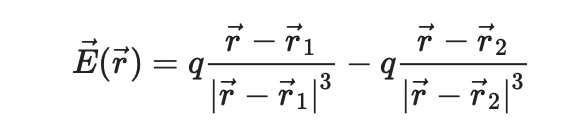
where 𝐸⃗ is the electric field vector, 𝑟⃗ is the position vector, and 𝑟⃗_1 and 𝑟⃗_2 are the locations of the two charges.

Visualization of the electric field

The electric field is a vector field, and to visualize it with matplotlib, we can use the quiver function.

import numpy as np
import matplotlib.pyplot as plt

# Define the function to calculate the electric field of an electric dipole
def electric_field(x, y, q, d):
    r1 = np.sqrt((x-d/2)**2 + y**2)
    r2 = np.sqrt((x+d/2)**2 + y**2)
    E_x = q * ((x-d/2)/r1**3 - (x+d/2)/r2**3)
    E_y = q * (y/r1**3 - y/r2**3)
    return E_x, E_y

# plot the vector field on a given figure (ax)
def make_field_plot(ax, npoints, **kwargs):
        
    # Define the domain of the electric field
    x = np.linspace(*lims, npoints)
    y = np.linspace(*lims, npoints)
    X, Y = np.meshgrid(x, y)
    # Calculate the electric field at each point in the domain
    E_x, E_y = electric_field(X, Y, q, d)
    # Calculate the length of the electric field vectors
    E_norm = np.sqrt(E_x**2 + E_y**2)
    # Normalize the electric field vectors to a fixed length
    E_x_norm = E_x / E_norm
    E_y_norm = E_y / E_norm
    # Plot the electric field vectors
    ax.quiver(X, Y, E_x_norm, E_y_norm, pivot='mid', **kwargs)
    
# Define the position and charge of the electric dipole
d = 2.0
q = 1.0

# Create a figure and axis object
fig, ax = plt.subplots()
lims = (-2, 2)

make_field_plot(ax, 14)

# Plot the charges
ax.plot([-d/2], [0], 'o', color='red')
ax.plot([d/2], [0], 'o', color='blue')

# Set the title and axis labels of the plot
ax.set_title('Electric Field of an Electric Dipole')
ax.set_xlabel('x')
ax.set_ylabel('y')

# Set the limits of the axis
ax.set_xlim(*lims)
ax.set_ylim(*lims)

# Set the aspect ratio
ax.set_aspect('equal')

# Show the plot
plt.show()

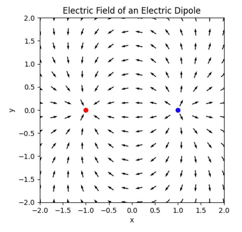
The quiver function takes at least four arguments: X, Y, U, and V.

X and Y are the coordinates of the points where the electric field vectors are plotted. In the code, X and Y are generated using the np.meshgrid function to create a grid of points in the domain of the electric field. U and V correspond to the directions of the arrows. Here, they are the components of the electric field vectors at each point. These are calculated using the electric_field function, which takes the X and Y coordinates, as well as the distance d and charge q of the dipole. Additionally, the pivot argument is set to 'mid', which means that the electric field vectors are anchored at their midpoints.

In addition to these arguments, there are many other options that can be passed as keyword arguments to control the appearance of the vectors and the plot as a whole. Some of these include:

• alpha: the transparency of the vectors.
• units: the units of the vector components.
• angles: the angle convention used to rotate the vectors.
• headlength, headwidth, headaxislength: the size and shape of the arrowheads.
• cmap, norm: options for color mapping and normalization.

Check out the online help to tweak your vector field to look exactly as you like.

If you found this article useful, you may want to consider becoming a Medium member to get unlimited access to all Medium articles. By registering using this link you can even support me as a writer.