Summary

The article demonstrates the application of Support Vector Machine (SVM) for classification tasks using the Iris dataset in Python, showcasing the SVM's ability to handle both linearly and non-linearly separable data through the use of kernels, particularly the Radial Basis Function (RBF).

Abstract

In the article, the author builds upon a previous introduction to Support Vector Machine (SVM) by illustrating its practical implementation in Python. The Iris dataset is utilized to visualize SVM's effectiveness, starting with a subset of the data that is linearly separable. The author explains the concept of support vectors and their significance in defining the decision boundary. Through code examples and visualizations, the article shows how to train an SVM model, identify support vectors, and visualize the decision boundary. The author then transitions to demonstrating SVM's capability to classify non-linearly separable data by introducing the kernel trick, specifically using the RBF kernel. This technique allows the SVM to implicitly map data to a higher-dimensional space where a linear separation is possible, thus solving a complex classification problem without the need for explicit additional dimensions. The article concludes by emphasizing the power and simplicity of SVM with kernel functions, which can transform a non-linear problem into a linear one by adjusting a single model parameter.

Opinions

The author emphasizes the importance of support vectors in SVM, noting that only these points influence the final decision boundary parameters.
The article conveys the robustness of SVM in handling complex classification tasks, particularly through the use of kernel functions like RBF.
The author suggests that the kernel trick is a computationally efficient method for dealing with non-linear data, as it avoids the need to explicitly compute higher-dimensional representations.
The article implies that SVM with the RBF kernel is a powerful tool for practitioners, as it can effectively classify data that cannot be separated by a straight line in two dimensions.
The author's use of the Iris dataset to demonstrate SVM's capabilities indicates a preference for well-known benchmark datasets to illustrate machine learning concepts.

Visualizing SVM with Python

In my previous article, I introduced the idea behind the classification algorithm Support Vector Machine. Here, I’m going to show you a practical application in Python of what I’ve been explaining, and I will do so by using the well-known Iris dataset.

Following the same structure of that article, I will first deal on linearly separable data, then I will move towards no-linearly separable data, so that you can appreciate the power of SVM which lie in the so-called Kernel Trick.

Linearly-Separable Data

For this purpose, I’m going to use only two features and two classes of the Iris dataset (which contains 4 features and 3 classes). To do so, let’s first have a look at the correlation among features, so that we can pick those features and classes which guarantee a linearly-separable demo dataset.

import seaborn as sns
iris = sns.load_dataset("iris")
print(iris.head())
y = iris.species
X = iris.drop('species',axis=1)

sns.pairplot(iris, hue="species",palette="bright")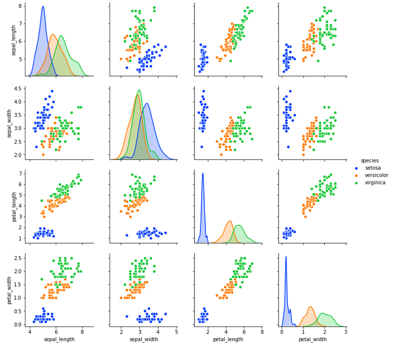

Since I first want to deal with linearly separable and two-class data, I will focus on the graph petal_width-petal_length, for the classes Setosa and Versicolor.

Let’s visualize it in the form we are going to use:

df=iris[(iris['species']!='virginica')]
df=df.drop(['sepal_length','sepal_width'], axis=1)
df.head()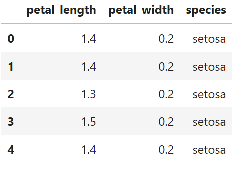

#let's convert categorical values to numerical target

df=df.replace('setosa', 0)
df=df.replace('versicolor', 1)

X=df.iloc[:,0:2]
y=df['species']
plt.scatter(X.iloc[:, 0], X.iloc[:, 1], c=y, s=50, cmap='autumn')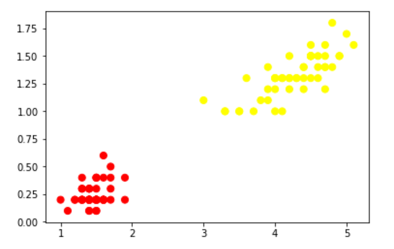

Nice, now let’s train our algorithm:

from sklearn.svm import SVC 
model = SVC(kernel='linear', C=1E10)
model.fit(X, y)

We can also call and visualize the coordinates of our support vectors:

model.support_vectors_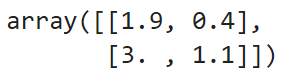

plt.scatter(X.iloc[:, 0], X.iloc[:, 1], c=y, s=50, cmap='autumn')
plt.scatter(model.support_vectors_[:,0],model.support_vectors_[:,1])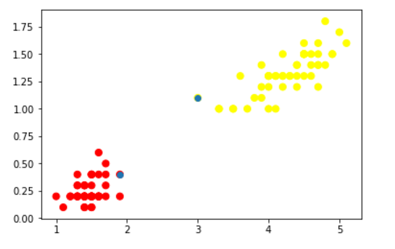

Now let’s visualize all the elements of our algorithm:

ax = plt.gca()

plt.scatter(X.iloc[:, 0], X.iloc[:, 1], c=y, s=50, cmap='autumn')

xlim = ax.get_xlim()
ylim = ax.get_ylim()

xx = np.linspace(xlim[0], xlim[1], 30)
yy = np.linspace(ylim[0], ylim[1], 30)
YY, XX = np.meshgrid(yy, xx)
xy = np.vstack([XX.ravel(), YY.ravel()]).T
Z = model.decision_function(xy).reshape(XX.shape)

ax.contour(XX, YY, Z, colors='k', levels=[-1, 0, 1], alpha=0.5,
           linestyles=['--', '-', '--'])

ax.scatter(model.support_vectors_[:, 0], model.support_vectors_[:, 1], s=100,
           linewidth=1, facecolors='none', edgecolors='k')
plt.show()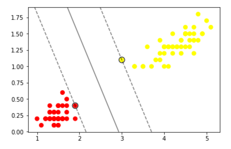

As you can see, our algorithm found those coefficients for our hyperplane which maximize the margin.

If you recall, in my last article I’ve been talking about the importance of Support Vectors. These points define a very interesting property of SVM optimization problem: only a few points actually end up in the final solution for creating the vector of parameters w which will define the best hyperplane. Hence, every point that is not a support vector can be moved anytime you want, yet it will not affect our decision boundary parameters.

Here, I’m going to show you the proof of this property, by reducing the size of our sample (yet without removing support vectors).

red_sample=df.sample(frac=0.7)
X=red_sample.iloc[:,0:2]
y=red_sample['species']
plt.scatter(X.iloc[:, 0], X.iloc[:, 1], c=y, s=50, cmap='autumn')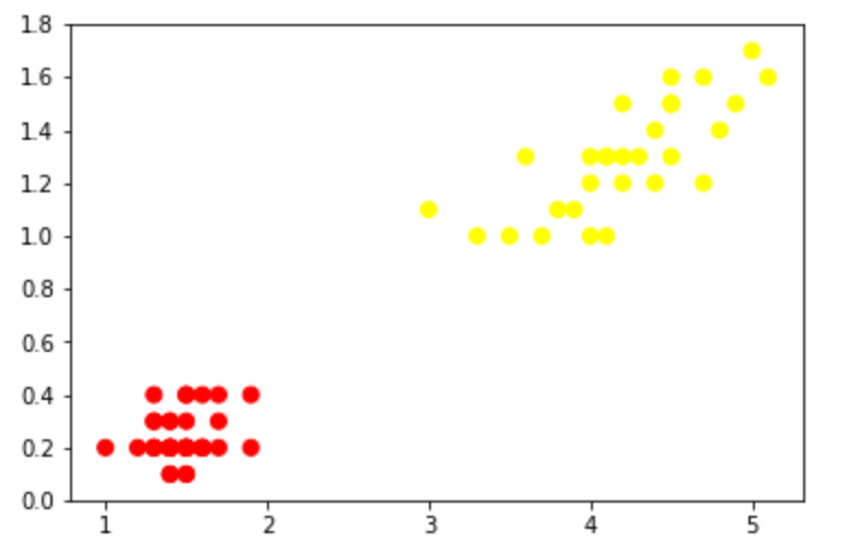

Now, if we train again our SVM here, knowing that the two support vectors are still there, we will obtain exactly the same hyperplane:

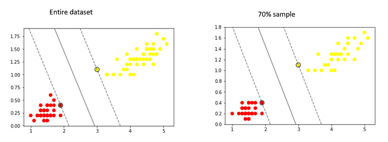
That’s because, again, only data which are support vectors end up building the best hyperplane.

Now I’m going to move to no-linearly separable data.

No-Linearly-Separable Data

For this purpose, I’m going to manually generate some no-linearly separable data. I’m doing so, rather than using the previous dataset, so that you can see the kernel function we are going to use (the Radial Basis Function) perfectly working.

from sklearn.datasets.samples_generator import make_circles
X, y = make_circles(100, factor=.1, noise=.1)

plt.scatter(X[:, 0], X[:, 1], c=y, s=50, cmap='autumn')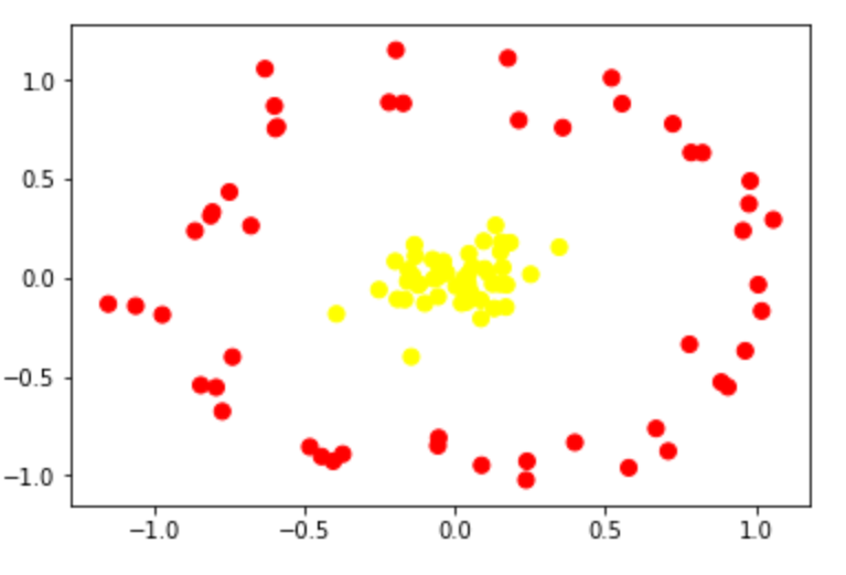

As you can see, data cannot be segregated by a straight line. Indeed, by using the same linear kernel of above, we obtain the following:

model=SVC(kernel='linear').fit(X, y)

ax = plt.gca()

xlim = ax.get_xlim()
ylim = ax.get_ylim()

# create grid to evaluate model
xx = np.linspace(xlim[0], xlim[1], 30)
yy = np.linspace(ylim[0], ylim[1], 30)
YY, XX = np.meshgrid(yy, xx)
xy = np.vstack([XX.ravel(), YY.ravel()]).T
Z = model.decision_function(xy).reshape(XX.shape)

# plot decision boundary and margins
ax.contour(XX, YY, Z, colors='k', levels=[-1, 0, 1], alpha=0.5,
           linestyles=['--', '-', '--'])
# plot support vectors
ax.scatter(model.support_vectors_[:, 0], model.support_vectors_[:, 1], s=100,
           linewidth=1, facecolors='none', edgecolors='k')
plt.show()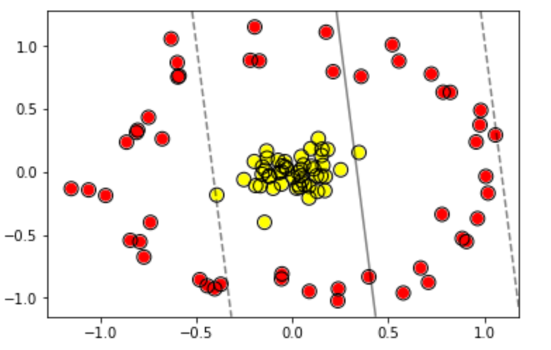

However, if we were able to move from a 2D to a 3D task, we would be able to lift all the yellow points and then use a plan to segregate the two clouds of points:

from mpl_toolkits import mplot3d

#setting the 3rd dimension with RBF centered on the middle clump

r = np.exp(-(X ** 2).sum(1))

ax = plt.subplot(projection='3d')
ax.scatter3D(X[:, 0], X[:, 1], r, c=y, s=50, cmap='autumn')
ax.set_xlabel('x')
ax.set_ylabel('y')
ax.set_zlabel('r')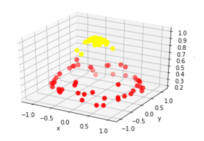

By doing so, we could separate those two classes with a plan. However, working with 3-dimensions on huge datasets is computationally costly in terms of speed. Furthermore, we should make sure that the elevation function we computed (our r) is the one which best put far apart our two classes.

Luckily, we do not need to worry about these pitfalls, we don’t even have to compute the third dimension. It is implicitly done by our SVM algorithm through the kernel trick, and it is done in such a way that the two caveats above are bypassed.

So, if we simply fit our model with kernel=rbf rather than kernel=linear:

model=SVC(kernel='rbf').fit(X, y)

we obtain the following:

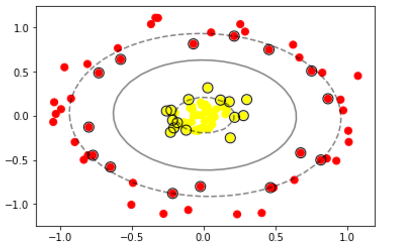
As you can see, without making any further computation, but simply changing one parameter of our model, we converted a no-linear problem to a linear one, thanks to the kernel trick.