Verifying the Assumptions of Linear Regression in Python and R

Dive deeper into the Gauss-Markov Theorem and other assumptions of linear regression!

Linear regression is one of the most basic machine learning algorithms and is often used as a benchmark for more advanced models. I assume the reader knows the basics of how linear regression works and what a regression problem is in general. That is why in this short article I would like to focus on the assumptions of the algorithm — what they are and how we can verify them using Python and R. I do not try to apply the solutions here but indicate what they could be.

In this article, I mainly use Python (in Jupyter Notebook), but I also show how to use rpy2 — an ‘interface between both languages to benefit from the libraries of one language while working in the other’. It enables us to run both R and Python in the same Notebook and even transfer objects between the two. Intuitively, we need to have R installed on our computer as well.

Disclaimer: Some of the cells using rpy2 do not work and I have to ‘cheat’ by running them in R to show the results. This is mostly the case for cells using ggplot2. Nonetheless, I leave the code in this cell. Let me know in the comments if this works for you :)

Let’s start!

1. Data

For this article, I use a classic regression dataset — Boston house prices. For simplicity, I only take the numeric variables. That’s why I drop the only boolean feature — CHAS. I am not going to go deeper into the meaning of the features, but this can always be inspected by running print(boston.DESCR).

2. Running Linear Regression

Most readers would probably estimate a linear regression model like this:

Coefficients: [-1.13139078e-01  4.70524578e-02  4.03114536e-02 -1.73669994e+01
  3.85049169e+00  2.78375651e-03 -1.48537390e+00  3.28311011e-01
 -1.37558288e-02 -9.90958031e-01  9.74145094e-03 -5.34157620e-01]
Intercept: 36.89195979693238
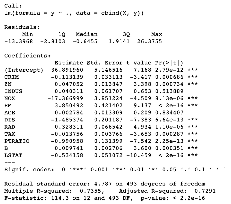
R^2 score: 0.7355165089722999

Which is of course not a wrong approach. However, coming to Python from R, I had a bit higher expectations about the amount of information I receive by default. To run R inside our Notebook we first need to run the magic command:

%load_ext rpy2.ipython

Afterward, using another magic command indicate that the cell contains R code. At this step, I also use the input command -i to indicate that I am passing an object from Python to R. To retrieve the output from R to Python we can use -o. Running the two lines results in much more information, including statistical significance and some metrics like R².

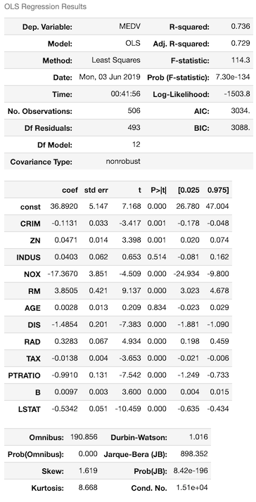
Of course, Python does not stay behind and we can obtain a similar level of details using another popular library — statsmodels. One thing to bear in mind is that when using linear regression in statsmodels we need to add a column of ones to serve as intercept. For that I use add_constant. The results are much more informative than the default ones from sklearn.

So now we see how to run linear regression in R and Python. Let’s continue to the assumptions. I break these down into two parts:

• assumptions from the Gauss-Markov Theorem
• rest of the assumptions

3. Gauss-Markov Theorem

During your statistics or econometrics courses, you might have heard the acronym BLUE in the context of linear regression. What was the meaning of it? According to the Gauss–Markov theorem, in a linear regression model the ordinary least squares (OLS) estimator gives the best linear unbiased estimator (BLUE) of the coefficients, provided that:

• the expectation of errors (residuals) is 0
• the errors are uncorrelated
• the errors have equal variance — homoscedasticity of errors

Also, ‘best’ in BLUE means resulting in the lowest variance of the estimate, in comparison to other unbiased, linear estimators.

For the estimator to be BLUE, the residuals do not need to follow normal (Gaussian) distribution, nor do they need to be independent and identically distributed.

Linearity of the model

The dependent variable (y) is assumed to be a linear function of the independent variables (X, features) specified in the model. The specification must be linear in its parameters. Fitting a linear model to data with non-linear patterns results in serious prediction errors, especially out-of-sample (data not used for training the model).

To detect nonlinearity one can inspect plots of observed vs. predicted values or residuals vs. predicted values. The desired outcome is that points are symmetrically distributed around a diagonal line in the former plot or around a horizontal line in the latter one. In both cases with a roughly constant variance.

Observing a ‘bowed’ pattern indicates that the model makes systematic errors whenever it is making unusually large or small predictions. When the model contains many features, nonlinearity can also be revealed by systematic patterns in plots of the residuals vs. individual features.

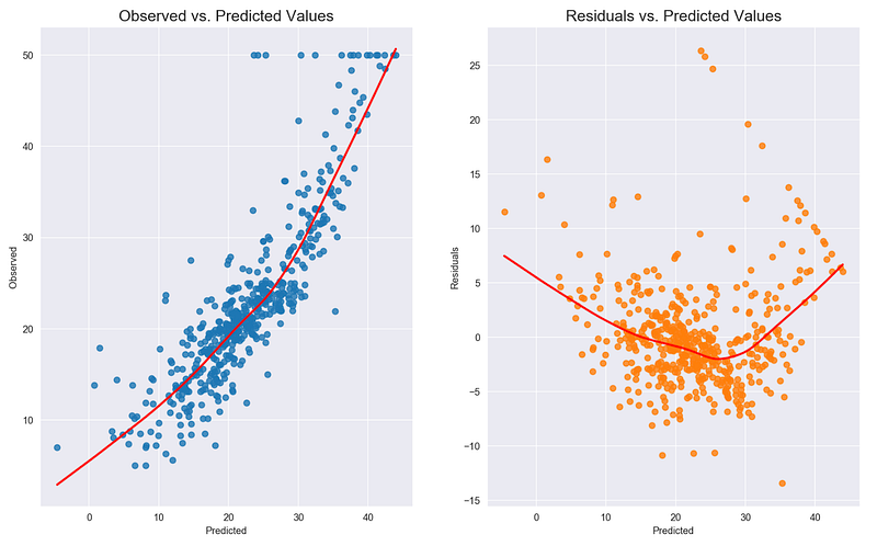
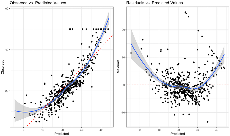
The inspection of the plots shows that the linearity assumption is not satisfied.

Potential solutions:

• non-linear transformations to dependent/independent variables
• adding extra features which are a transformation of the already used ones (for example squared version)
• adding features that were not considered before

Expectation (mean) of residuals is zero

This one is easy to check. In Python:

lin_reg.resid.mean()
# -1.0012544153465325e-13

And in R:

%%R
mean(lin_reg$resid)
# 2.018759e-17

The results are a bit different, as far as I know, this is a numeric approximation issue. However, we can assume that the expectation of residuals is indeed 0.

No (perfect) multicollinearity

In other words, the features should be linearly independent. What does that mean in practice? We should not be able to use a linear model to accurately predict one feature using another one. Let’s take X1 and X2 as examples of features. It could happen that X1 = 2 + 3 * X2, which violates the assumption.

One scenario to watch out for is the ‘dummy variable trap’ — when we use dummy variables to encode a categorical feature and do not omit the baseline level from the model. This results in a perfect correlation between the dummy variables and the constant term.

Multicollinearity can be present in the model, as long as it is not ‘perfect’. In the former case, the estimates are less efficient but still unbiased. The estimates will be less precise and highly sensitive to particular sets of data.

We can detect multicollinearity using the variance inflation factor (VIF). Without going into too many details, the interpretation of VIF is as follows: the square root of a given variable’s VIF shows how much larger the standard error is, compared with what it would be if that predictor were uncorrelated with the other features in the model. If no features are correlated, then all values for VIF will be 1.

%%R
library(car)
vif(lin_reg)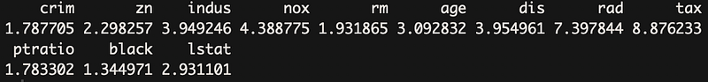

To deal with multicollinearity we should iteratively remove features with high values of VIF. A rule of thumb for removal could be VIF larger than 10 (5 is also common). Another possible solution is to use PCA to reduce features to a smaller set of uncorrelated components.

Tip: we can also look at the correlation matrix of features to identify dependencies between them.

Homoscedasticity (equal variance) of residuals

When residuals do not have constant variance (they exhibit heteroscedasticity), it is difficult to determine the true standard deviation of the forecast errors, usually resulting in confidence intervals that are too wide/narrow. For example, if the variance of the residuals is increasing over time, confidence intervals for out-of-sample predictions will be unrealistically narrow. Another effect of heteroscedasticity might also be putting too much weight to a subset of data when estimating coefficients — the subset in which the error variance was largest.

To investigate if the residuals are homoscedastic, we can look at a plot of residuals (or standardized residuals) vs. predicted (fitted) values. What should alarm us is the case when the residuals grow either as a function of predicted value or time (in case of time series).

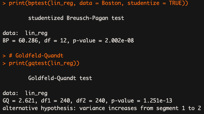
We can also use two statistical tests: Breusch-Pagan and Goldfeld-Quandt. In both of them, the null hypothesis assumes homoscedasticity and a p-value below a certain level (like 0.05) indicates we should reject the null in favor of heteroscedasticity.

In the snippets below I plot residuals (and standardized ones) vs. fitted values and carry out the two mentioned tests. To identify homoscedasticity in the plots, the placement of the points should be random and no pattern (increase/decrease in values of residuals) should be visible — the red line in the R plots should be flat. We can see that this is not the case for our dataset.

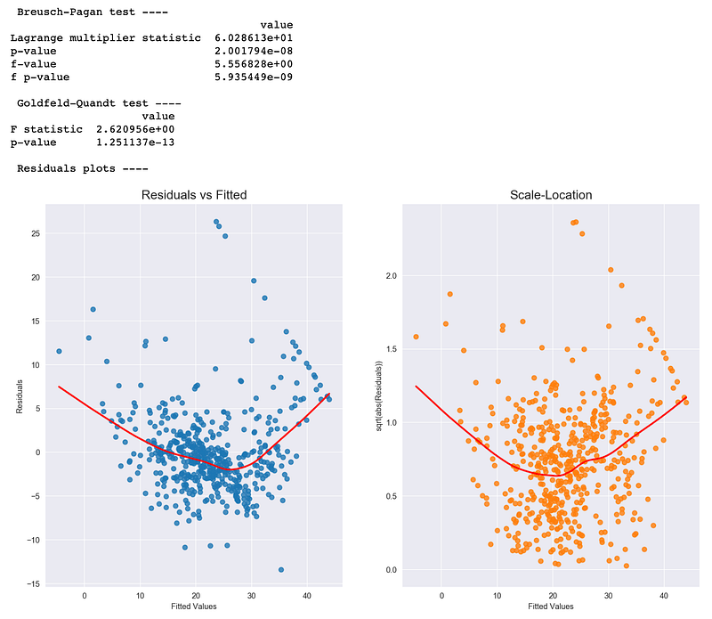
The results indicate that the assumption is not satisfied and we should reject the hypothesis of homoscedasticity.

Potential solutions:

• log transformation of the dependent variable
• in case of time series, deflating a series if it concerns monetary value
• using ARCH (auto-regressive conditional heteroscedasticity) models to model the error variance. An example might be stock market, where data can exhibit periods of increased or decreased volatility over time (volatility clustering, see this article for more information)

No autocorrelation of residuals

This assumption is especially dangerous in time-series models, where serial correlation in the residuals implies that there is room for improvement in the model. Extreme serial correlation is often a sign of a badly misspecified model. Another reason for serial correlation in the residuals could be a violation of the linearity assumption or due to bias that is explainable by omitted variables (interaction terms or dummy variables for identifiable conditions). An example of the former case might be fitting a (straight) line to data, which exhibits exponential growth over time.

This assumption also has meaning in the case of non-time-series models. If residuals always have the same sign under particular conditions, it means that the model systematically underpredicts/overpredicts what happens when the predictors have a particular configuration.

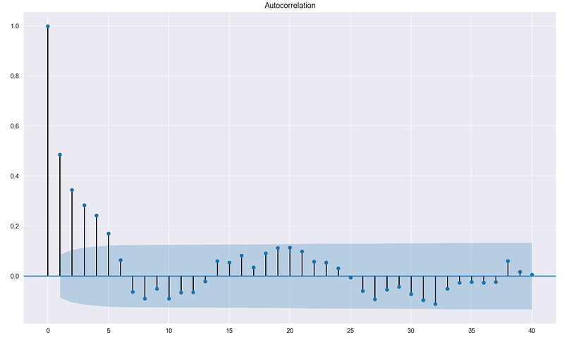
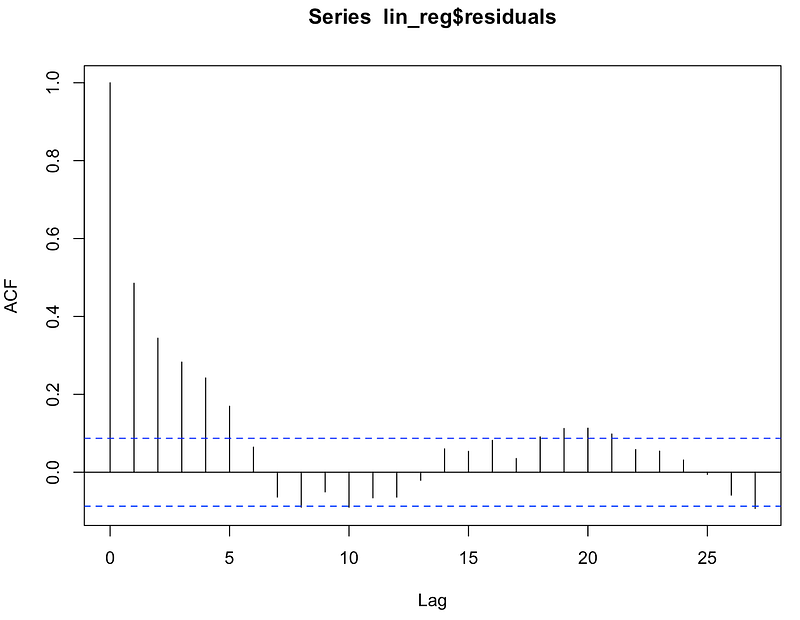
To investigate if autocorrelation is present, I use ACF (autocorrelation function) plots and Durbin-Watson test.

In the former case, we want to see if the value of ACF is significant for any lag (in case of no time-series data, the row number is used). While calling the function, we indicate the significance level (see this article for more details) we are interested in and the critical area is plotted on the graph. Significant correlations lie outside of that area.

Note: when dealing with data without the time dimension, we can alternatively plot the residuals vs. the row number. In such cases, rows should be sorted in a way that (only) depends on the values of the feature(s).

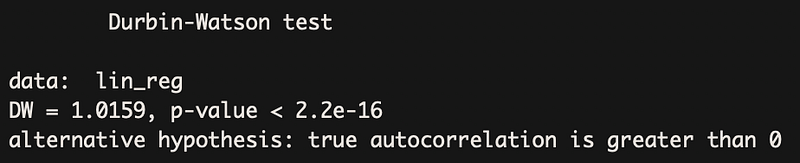
The second approach is using the Durbin-Watson test. I do not go into detail how it is constructed but provide a high-level overview. The test statistic provides a test for significant residual autocorrelation at lag 1. The DW statistic is approximately equal to 2(1-a), where a is the lag 1 residual autocorrelation. The DW test statistic is located in the default summary output of statsmodels’s regression.

Some notes on the Durbin-Watson test:

• the test statistic always has a value between 0 and 4
• value of 2 means that there is no autocorrelation in the sample
• values < 2 indicate positive autocorrelation, values > 2 negative one.

Potential solutions:

• in case of minor positive autocorrelation, there might be some room for fine-tuning the model, for example, adding lags of the dependent/independent variables
• some seasonal components might not be captured by the model, account for them using dummy variables or seasonally adjust the variables
• if DW < 1 it might indicate a possible problem in model specification, consider stationarizing time-series variables by differencing, logging, and/or deflating (in case of monetary values)
• in case of significant negative correlation, some of the variables might have been overdifferenced
• use Generalized Least Squares
• include a linear (trend) term in case of a consistent increasing/decreasing pattern in the residuals

4. Other assumptions

Below I present some of the other commonly verified assumptions of linear regression.

The features and residuals are uncorrelated

To investigate this assumption I check the Pearson correlation coefficient between each feature and the residuals. Then report the p-value for testing the lack of correlation between the two considered series.

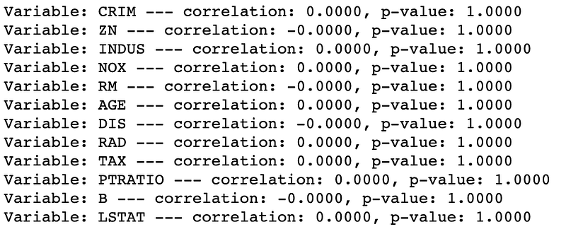
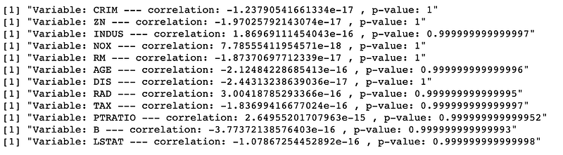
I cannot reject the null hypothesis (lack of correlation) for any pair.

The number of observations must be greater than the number of features

This one is pretty straightforward. We can check the shape of our data by using shape method in Python or dim function in R. Also, a rule of thumb says that we should have more than 30 observations in the dataset. This is taken from the Central Limit Theorem, which states that adding IID random variable results in a normalized distribution when the sample size is greater than 30, even when the random variables are not Gaussian themselves.

There must be some variability in features

This assumption states that there must be some variance in the features, as a feature that has a constant value for all or the majority of observations might not be a good predictor. We can check this assumption by simply checking the variance of all features.

X.apply(np.var, axis=0)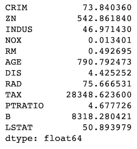

In caret package in R there is a function called nearZeroVar for identifying features with zero or near-zero variance.

%%R
library(caret)

apply(X, 2, var)
nearZeroVar(X, saveMetrics= TRUE)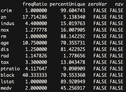

Normality of residuals

When this assumption is violated, it causes problems with calculating confidence intervals and various significance tests for coefficients. When the error distribution significantly departs from Gaussian, confidence intervals may be too wide or too narrow.

Some of the potential reasons causing non-normal residuals:

• presence of a few large outliers in data
• there might be some other problems (violations) with the model assumptions
• another, better model specification might be better suited for this problem

Technically, we can omit this assumption if we assume instead that the model equation is correct and our goal is to estimate the coefficients and generate predictions (in the sense of minimizing mean squared error).

However, normally we are interested in making valid inferences from the model or estimating the probability that a given prediction error will exceed some threshold in a particular direction. To do so, the assumption about the normality of residuals must be satisfied.

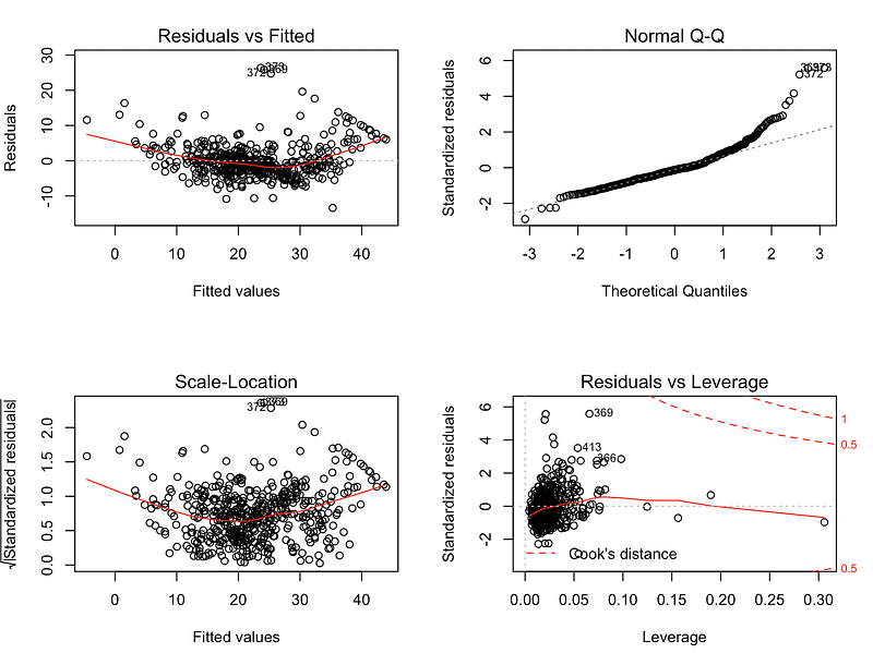
To investigate this assumption we can look at:

• QQ plots of the residuals (a detailed description can be found here). For example, a bow-shaped pattern of deviations from the diagonal implies that the residuals have excessive skewness (i.e., the distribution is not symmetrical, with too many large residuals in one direction). The s-shaped pattern of deviations implies excessive kurtosis of the residuals — there are either too many or two few large errors in both directions.
• use statistical tests such as the Kolmogorov-Smirnov test, the Shapiro-Wilk test, the Jarque-Bera test, and the Anderson-Darling test

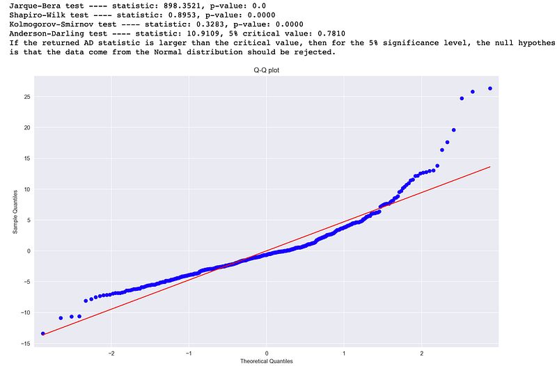
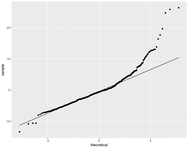
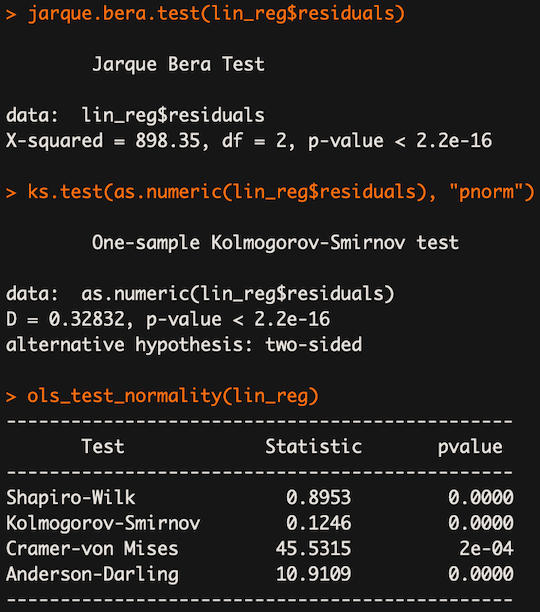
From the results above we can infer that the residuals do not follow Gaussian distribution — from the shape of the QQ plot, as well as rejecting the null hypothesis in all statistical tests. The reason why Kolmogorov-Smirnov from ols_test_normality shows different results is that it does not run the `two-sided` version of the test.

Potential solutions:

• nonlinear transformation of target variable or features
• remove/treat potential outliers
• it can happen that there are two or more subsets of the data having different statistical properties, in which case separate models might be considered

5. Bonus: Outliers

This is not really an assumption, however, the existence of outliers in our data can lead to violations of some of the above-mentioned assumptions. That is why we should investigate the data and verify if some extreme observations are valid and important for our research or merely some errors which we can remove.

I will not dive deep into outlier detection methods as there are already many articles about them. A few potential approaches:

• Z-score
• box plot
• Leverage — a measure of how far away the feature values of a point are from the values of the different observations. The high-leverage point is a point at extreme values of the variables, where the lack of nearby observations makes the fitted regression model pass close to that particular point.
• Cook’s distance — a measure of how deleting an observation impacts the regression model. It makes sense to investigate points with high Cook’s distances.
• Isolation Forest — for more details see this article

6. Conclusions

In this article, I showed what are the assumptions of linear regression, how to verify if they are satisfied and what are potential steps we can take to fix the underlying issues with the model. The code used for this article can be found on GitHub.

As always, any constructive feedback is welcome. You can reach out to me on Twitter or in the comments.

Liked the article? Become a Medium member to continue learning by reading without limits. If you use this link to become a member, you will support me at no extra cost to you. Thanks in advance and see you around!

References

1. http://people.duke.edu/~rnau/testing.htm