Variational Gaussian Process (VGP) — What To Do When Things Are Not Gaussian

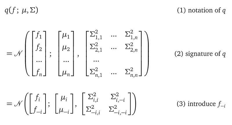
People may have the impression that Bayesian methods only work effectively when everything is Gaussian. That’s not true. Modern Bayesian machine learning can comfortably handle non-Gaussian distributions.

I will describe the Gaussian Process binary classification model. It uses a Gaussian prior but a Bernoulli likelihood. I will explain why a Bernoulli distribution prevents us from using the Bayes rule to compute the posterior. We call such posteriors intractable. Intractable or not, we need posteriors to make predictions. Then I will present the solution — variational inference — to approximate intractable posteriors.

The binary classification problem

We have some training data (X, Y):

X are real values; Y are binary values as labels. The task is to design a model that predicts the label Y from input X. This is a binary classification problem. Let’s plot the data and think about how to use Gaussian Process to build a binary classifier:

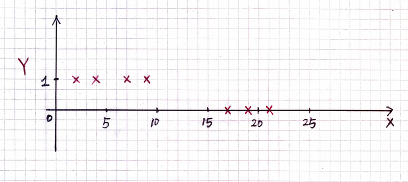
In the above figure, red crosses show the training data points. We realize there is a problem if we use Gaussian Process regression to model the data: Gaussian Process regression models continuous functions f(x). We cannot require such a function to return only 1 or 0. A Gaussian Process regression model may return 1.1 at some x locations, and 0.3 at other locations.

This problem is easy to solve. We use the Bernoulli distribution to model binary outputs. The Bernoulli distribution has a single parameter — the probability between 0 and 1, that describes how likely an event happens. To create a connection between this probability and our Gaussian Process function f(x), we define the function g(f(x)) that squashes the real-valued Gaussian Process function f(x) into a value in the range [0, 1].

g defined this way is a function of x. Just like when you have f(x) = x+1 and define g(f(x)) = f(x)², then g is a function of x: g(x) = (x+1)².

Many squashing functions (check sigmoid functions) work, and we choose the logit function because it is widely used and its mathematical property is easy to interpret:

The following figure illustrates this idea:

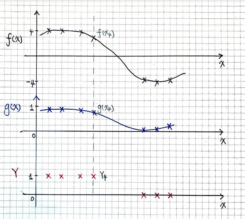
This figure has three parts:

1. The top part is a Gaussian Process function f(x) in black. It goes through some big real values (relatively to the range [0, 1]) at x locations where the corresponding label is 1. And it goes through some small values at x locations where the corresponding label is 0.
2. The middle part shows the g(x) function in blue. It squashes the values of the f(x) function to be in the range [0, 1].
3. The bottom part shows our training data in red.

Let’s run through an example data point — data point (X₄=9, Y₄=1) highlighted in the figure. For this point, the top part reads f(9)=3. In the middle part, the squashing function g(9) is:

With 0.98 being its parameter, the Bernoulli distribution says the probability of Y₄=1 is 0.98. According to the bottom part, the label Y₄ is indeed 1. This model is good.

By the way, this idea of using a squashing function is very similar to how we build a neural network classifier: a softmax function turns the output value (a value in the full real line) of the neurons in the last hidden layer into probabilities between 0 and 1.

Encouraged by this example, we formally define this Bayesian model. But first, some notations.

Some notations

Medium supports Unicode in text. This allows me to write many math subscript notations such as X₁ and Xₙ. But I could not write down some other subscripts. For example:

So in the text, I will use an underscore “_” to lead such subscripts, such as X_* and X_*1.

If some math notations render as question marks on your phone, please try to read this article from a computer. This is a known issue with some Unicode rendering.

The binary classification model

A Bayesian model always consists of two parts: the prior and the likelihood.

The prior

As the name may suggest, the Gaussian Process prior is always a multivariate Gaussian distribution. It models the function at the top of the previous figure. To refresh your memory, take a look at Understanding Gaussian Process, the Socratic Way.

The GP prior is a joint multivariate Gaussian distribution between two random variable vectors f(X) and f(X_*):

• f(X) is a random variable vector of length n, with n being the number of training data points. f(X) represents function values at training locations X.
• f(X_*) is another random variable vector. It represents function values at testing locations X_*, i.e. the locations where you want your model to make a prediction. The length of f(X_*) is the same as the number of testing locations X_*.

I use f as a shorthand for f(X). And fᵢ for the i-th random variable in this vector, which corresponds to the i-th training data point. Similarly, f_* is a shorthand for f(X_*).

The GP prior uses the following kernel function k(x, x′) to define the correlation between two individual random variables f(x) at location x and f(x′) at location x′ (both x and x′ can be in the location set X or X_*):

where exp is the exponential function. l and σ² are kernel parameters. l is called the lengthscale, and σ² the signal variance. l and σ² are scalars. Since they are parameters that we introduce to the model, we also call them model parameters. The kernel function k mentions our training location X in the covariance block k(X, X), and testing location X_* in the covariance block k(X_*, X_*) and both X and X_* in k(X_*, X). k does not mention the training data Y.

In short, the GP prior introduces random variables f at training location and random variables f_* at testing locations and uses the kernel function k to define the correlation between any two individual random variables. This correlation enables the model to reason about the value of random variables at testing locations by using the information of the random variables at training locations, in order words, to make predictions.

Even though the GP prior is a joint distribution for f and f_*, only f has a connection to our training data. We can apply the multivariate Gaussian marginalization rule to the GP prior to derive the marginal distribution p(f) just for f. And a few paragraphs later, we will establish the connection from the training data Y to f via the likelihood.

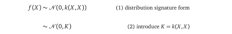
Below is the marginalized f, where K is a shorthand for k(X, X):

Or alternatively, in the form of the probability density function:

Compared to the notation p(f), the notation p(f; l, σ²) emphasizes that this distribution is over the random variables f; and mentions model parameters l and σ². They come from the exponential squared kernel function mentioned in K. det is the matrix determinant operator.

Note in this article, we don’t treat l and σ² as random variables. We treat them as scalar parameters of the model. Being a scalar, each model parameter can take a single concrete value, such as l=10.4. We don’t know this value now. I will introduce a parameter learning to find a single value for l (as well as for other model parameters). This concrete value is called a point estimate.

Other parameter learning methods exist, for example, we can treat l and σ² as random variables, which can take a distribution of values. This is called a full Bayesian treatment and is a topic of a future article.

The likelihood

Let’s introduce a new random variable vector y(X), which I shorten as y. We model our observations Y as samples of the random variables in y — each Yᵢ is a sample from the corresponding random variable yᵢ. y is of length n, with n being the number of training data points.

Since y are random variables for which we have observations, we call it an observational random variable. On the contrary, random variables f and f_* don’t have associated observations, we call them latent random variables.

The likelihood, denoted as p(y|f, f_*) is a conditional distribution. It describes the probability of the observational random variable y, given the latent variables f and f_* from the GP prior.

But we should not design our model such that random variables with observations depend on random variables without observations. So we enforce that y does not depend on f_*. This results in the likelihood p(y|f) by dropping the irrelevant f_* under the condition:

Since our observation Yᵢ is a binary value, we model it as a sample from a Bernoulli random variable yᵢ. The probability density function for yᵢ is:

with gᵢ being the only parameter of the Bernoulli distribution. gᵢ is a shorthand for the function application g(fᵢ). By plugging in the value Yᵢ for yᵢ, we can evaluate the probability of yᵢ taking that value. So y is a vector of Bernoulli random variables.

Let’s decipher the Bernoulli probability density further: gᵢ, which is a shorthand for g(fᵢ), represents the probability that the observational random variable yᵢ has the value 1. Since yᵢ can only take 0 or 1, the probability that yᵢ has the value 0 is 1-gᵢ. The above expression is a succinct form that combines these two cases into a single formula.

The above Bernoulli density function establishes the connection from the observation Yᵢ to the observational random variable yᵢ. And by invoking the function g with fᵢ as an argument, we established the connection from Yᵢ to fᵢ:

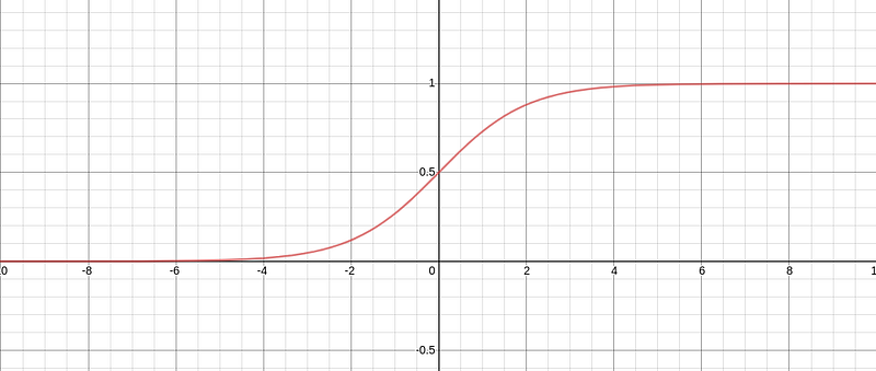
This function has the following shape, with x-axis plots fᵢ and y-axis plots g(fᵢ):

Let’s look at this likelihood function with full detail at a single location Xᵢ:

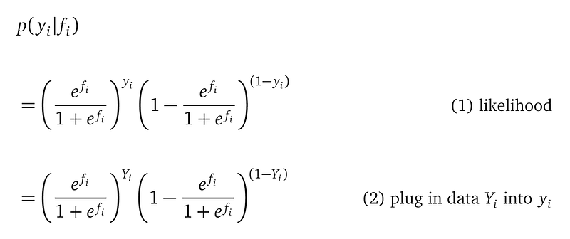
Line (1) is the full formula for the likelihood function at the single location Xᵢ, given the random variable fᵢ, which is from our GP prior.

Line (2) plugs in the actual observation Yᵢ into the random variable yᵢ.

This likelihood mentions our training data Yᵢ, but it does not mention the training data Xᵢ. Compare this to the GP prior, which mentions data Xᵢ but not Yᵢ. And the random variable fᵢ is the bridge between the prior and the likelihood that connects Xᵢ and Yᵢ together.

We would like our model to give a high value to the likelihood. So let’s analyze when the likelihood evaluates to a high value. Let’s focus on the case when Yᵢ=1 (the case Yᵢ=0 is similar). When Yᵢ=1, the likelihood simplifies to:

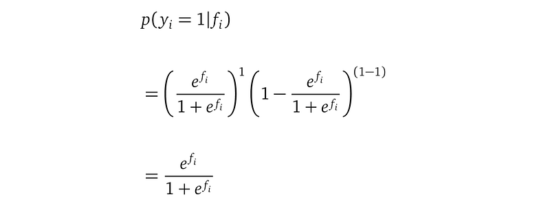
To make this quantity as high as possible (maximum is 1), we need fᵢ to have a larger mean, and hopefully a small variance. This way, the expected value of fᵢ is a large value. Transitively, the expected value of the above formula will be a value closer to 1, its maxima.

Note, we don’t care about the exact mean value for fᵢ. As long as the likelihood evaluates to a high probability number, we are happy, no matter the mean is 4 or 7. We can imagine that fᵢ regresses to some latent data space.

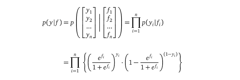
After we understood the likelihood of a single data point (Xᵢ, Yᵢ), it is easy to understand the likelihood of all the training data points. We assume that observations are independent of each other, so the likelihood for all the observational random variables p(y|f) is the product of all the n individual likelihoods, with n being the number of training data points:

Here, the likelihood p(y|f) does not mention any model parameters, l or σ². But in general, likelihood functions can introduce new model parameters.

Now you’ve learned how to incorporate non-Gaussian distributions into your likelihood. Similarly, you can introduce other non-Gaussian distribution, such as student-t to handle outliers.

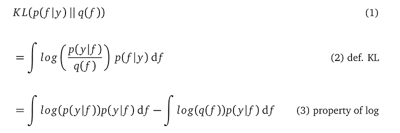
The posterior

After we described the prior p(f) and the likelihood p(y|f), it’s time for the posterior p(f|y). The Bayes rule gives us the probability density function of the posterior from the prior and the likelihood:

The posterior mentions our two model parameters l, σ². They come from the kernel function k inside the prior p(f). Sometimes we denote the posterior as p(f|y; l, σ²) to emphasize these model parameters.

The denominator is called marginal likelihood. It is an n-dimensional integration, each dimension is for a single random variable in the random variable vector f. We have to first compute the result of this integration then we can evaluate the posterior p(f|y) as a function, for example, to make predictions.

To compute the integration means to work out the analytical expression for the result of the integration. For example, we work out the result of ∫ x dx to be ½x². The expression ½x² is analytical — we can plug in a value of x to get the result of the integration.

However, we don’t know how to compute this integration. The function inside the integration symbol is the product between Bernoulli probability density function in p(y|f) and a multivariate Gaussian probability density function in p(f). You cannot find a rule from your Calculus book to work out this integration. People call it an intractable integration.

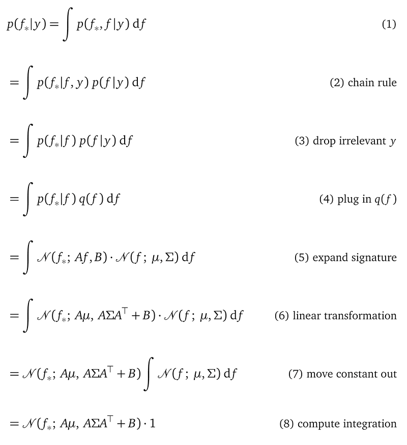
You may wonder, shouldn’t the posterior be a distribution over the same set of random variables f_* and f from the GP prior? So instead of p(f|y), the posterior should be p(f_*, f|y), no? You are right. But working with p(f|y) is all we need, because:

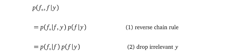
In other words, we decided to factorize the joint posterior p(f_*, f|y) into a conditional probability p(f_*|f) and a marginal probability p(f|y). And we know the formula for p(f_*|f) by applying the multivariate Gaussian conditional rule to the GP prior. So we only need to work with p(f|y).

Variational inference

We don’t know how to derive the analytical expression for the posterior p(f|y), in other words, we don’t know the structure of the posterior. The next best thing is to approximate the posterior with another distribution whose structure is in our control. So by design, we know the analytical expression for this new distribution’s probability density function.

Note we want to use a new distribution to approximate the posterior p(f|y), not to approximate the marginal likelihood p(y) = ∫ p(y|f) p(f) df. The posterior is a probability distribution over f. We need this distribution to make predictions. The marginal likelihood is a number introduced in the right-hand side of the Bayes rule to make sure the left-hand side is a proper probability density function that integrates to 1. When we use a new distribution to approximate the posterior p(f|y), we inherently take care of the marginal likelihood because this new distribution is proper by design.

Here is how I understand the phrase “approximating the posterior with another distribution”:

1. the probability density function of this new distribution is over the same set of random variables f as the posterior. So this new distribution can be plugged into places where the posterior appears.
2. This new distribution behaves similarly as the posterior. This means for a f, the new distribution returns a probability similar to the one that the true posterior would return. This way, the shape of the probability density function of this new distribution is similar to the posterior.

To understand the phrase “the new distribution’s structure is in our control”, let’s first develop this approximation concept further.

The variational distribution q

We call the distribution that we use to approximate the posterior the variational distribution. We use q(f) to denote its probability density function. What should q(f) look like?

We want q(f) to look like the posterior p(f|y), but we don’t know the structure of the posterior. How about we propose q to be a multivariate Gaussian distribution with mean μ and covariance matrix Σ?

The mean and covariance matrix fully decides the shape of a multivariate Gaussian distribution. As they change, the shape of the multivariate Gaussian distribution changes accordingly. So we can find concrete values for μ and Σ such that the shape of q(f) is similar to the shape of p(f|y). We use the notation q(f; μ, Σ) to emphasize these two parameters. We call them variational parameters.

The following figure illustrates the idea of making the shape of q(f; μ, Σ) to be close to the shape of p(f|y; l, σ²), with f being a single random variable, instead of a random variable vector:

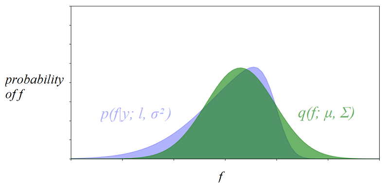
The purple distribution is irregularly shaped, illustrating the posterior whose structure we don’t know. The green distribution is bell-shaped, illustrating the variational distribution, which is a multivariate Gaussian. We tweak the values of μ and Σ to make the green overlaps with the purple as much as possible to make q(f; μ, Σ) approximate p(f|y).

Two very important assumptions that we take here:

1. We assume that there exist some concrete variational parameter values such that our multivariate Gaussian distribution q(f; μ, Σ) is similar to a non-Gaussian posterior p(f|y; l, σ²).
2. We assume that we can find at least one of these concrete values for μ and Σ by parameter learning.

Either assumption can be false in reality. So for some dataset, we may not be able to find good q(f) approximation for the posterior. This means we may not find a good Bayesian model to fit the training data well — the machine learning task has failed. This sucks, but it happens.

By the way, variational inference is very important in modern day machine learning, and is a topic that you won’t get away with. See its application in time series forecasting, and human face generation.

We control the shape of q through μ and Σ

Under the multivariate Gaussian proposal, the probability density function of q(f; μ, Σ) is:

where n is the number of training data points, det is the matrix determinant operator. Σ⁻¹ is the inverse of the covariance matrix Σ.

This formula also shows the importance of an analytical formula — it can be evaluated after plugging the concrete values for the unknowns: f, which is a float vector, μ, which is a float vector, and Σ, a float matrix of size n×n. When we have some concrete values of these three, the above formula evaluates to a single probability number — the probability of f under the multivariate Gaussian distribution.

The proposal for the variational distribution q to be a multivariate Gaussian seems to be pure guess now, but later you will see this structure has great advantages.

The variational distribution q(f; μ, Σ) has a fixed structure — the structure of a full multivariate Gaussian distribution. “full” means Σ is a dense matrix with no zeros. Let’s come back to that later in the Parameter learning section. What is important for us right now is that we can vary its shape by the two variational parameters μ and Σ. In theory, by changing the values of μ and Σ, we can get any possible Gaussian distribution over the random variable vector f. This is why q’s structure is in our control.

Once we decide the concrete values for μ and Σ, we will have the fully specified q that we can use as an approximation to the true posterior. But how do we decide which concrete values to assign to μ and Σ? The obvious answer is to choose values for μ and Σ such that q(f; μ, Σ) is as close to the posterior p(f|y, l, σ²) as possible.

We realize that we need a “closeness” measure from the distribution q(f) to the posterior p(f|y). And we need a way to minimize this closeness measure.

Kullback–Leibler divergence and the Evidence Lower Bound

Since we want our variational distribution q(f; μ, Σ) to be close to the posterior p(f|y; l, σ²), we need a closeness measure between them. We can use the Kullback–Leibler divergence (KL divergence) to define the closeness from one distribution to the other distribution. The formula for the KL divergence between the variational distribution q(f; μ, Σ) and the posterior p(f|y; l, σ²) is:

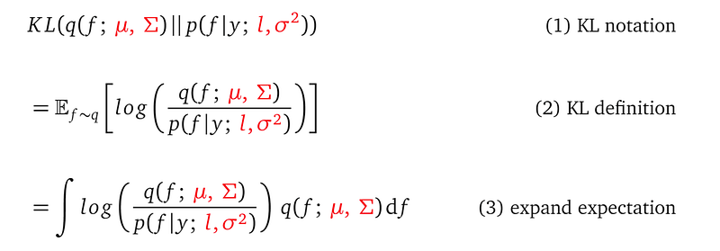
In the above derivations, I coloured the model parameters (both the kernel parameters and variational parameters)in red.

Line (1) is the notation for the KL divergence. The double vertical bar || inside the KL operator separates the two distributions that we want to compute the distance for.

Line (2) defines the meaning of the KL divergence. It is the expected log probability ratio between the two distributions. If for some f, q(f) and p(f|y) evaluate to the same probability, then their ratio is 1, and log(1) is 0. So this particular f does not contribute to the overall divergence measure. On the other hand, if this ratio is not 1, this f contributes to the final divergence measure. So KL divergence is the average difference between the probability densities for f in log scale.

Line (3) replaces the expectation with its mathematical computation — an integration. It shows the integrand (with training data X and Y plugged in) has 4 unknowns: l, σ², μ, Σ, which is the full set of model parameters. The random variable f is integrated out.

We want the shape of q(f; μ, Σ) to be as close to the shape of p(f|y; l, σ²) as possible. The KL divergence KL(q(f)||p(f|y)) encodes such closeness, and it is a function of the model parameters. The way to bring q(f) to be as close as p(f|y) is to minimize this KL divergence with respect to the model parameters:

There must be a question burning inside you — we don’t know the analytical form of the posterior p(f|y), how can we minimize the KL divergence that mentions it?

To answer this question, we need to keep manipulating the formula, but now I ignored the model parameters in the derivations to save space. Please remember, no matter how we manipulate the KL divergence between q(f) and p(f|y), it is always a function of the four model parameters.

At line (6), we don’t write the expectation operation around log p(y) because log p(y) does not mention the random variable f, and the ignored expectation is with respect to f. So the expectation evaluates to log p(y). We have a famous name for log p(y) — the log marginal likelihood.

The above derivation, especially line (6) confirms that we cannot compute this KL divergence. This is because it requires us to compute log marginal likelihood log p(y), but p(y) is the intractable integration that prevents us from using the Bayes rule to compute the posterior in the first place:

Since we cannot compute logp(y), let’s be brave and drop it and try to minimize the remaining two terms.

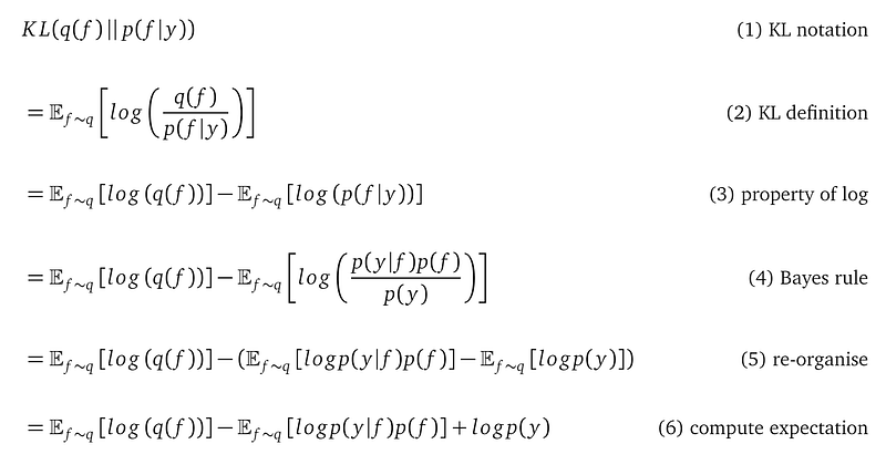
Equivalently, we can maximize the negation of these two terms. We give this negation a name Evidence Lower BOund, or ELBO:

Line (2) negates the first two terms from the above KL divergence formula and drops the third term log p(y), which we cannot compute.

Line (3) and line (4) re-organizes terms using the property of log and the linearity of the expectation, i.e. E[a+b] = E[a] + E[b] for two random variable a and b.

Line (5) recognizes that the second term is the KL-divergence between the variational distribution q(f) and the GP prior p(f).

Line (6) expands the expectation in the first term to its actual mathematical definition — an integration.

From now on, the ELBO will be the objective function that we maximize to bring the variational distribution q(f) to be as close to the posterior p(f|y).

Why it is ok to drop log p(y)?

With the EBLO defined, we have this equation:

Pay attention to the minus sign in front of the ELBO.

Our ideal goal is to minimize the KL(q(f)||p(f|y)), but since we cannot compute log p(y), we minimize -ELBO, or equivalently, maximize the ELBO as an alternative.

You may ask why it is ok to drop the log marginal likelihood log p(y)? To answer this question, I can quote “all models are wrong, but some are useful”. We know it is wrong to drop log p(y), but if we keep it, we cannot compute the formula.

Joking aside, I think the undertone of your question is: what information do we lose by dropping log p(y)? Can this information loss be tolerated so the remaining model still has the capacity to be useful? To answer this new question, let’s think what information log p(y) includes — it is a sum of likelihood p(y|f), weighted by the prior p(f):

The ELBO formula, shown again below, also includes information of the likelihood, which appears in the first term, and the prior, which appears in the second term:

So by dropping log p(y), we have not lost everything, that’s the important point. Sure, the remaining information does not appear in the form of a weighted sum, so we have some information loss. That’s the price we pay to use a computable alternative formula instead of an ideal, but uncomputable formula.

Intuition behind ELBO

We have an intuitive interpretation of ELBO by looking line (6) from above, which is copied here:

The first term is the expected likelihood with respect to the random variable f, now from the variational distribution q(f). The second term is the KL divergence between q(f) and the GP prior p(f) — note, not the posterior p(f|y), and remember a KL divergence is non-negative.

We want to maximize ELBO. To do that, we need the expected likelihood to be large, and the KL distance to be small. This mathematical meaning matches our intention well:

• we want our model q(f) to explain the training data well, through a large likelihood.
• At the same time, we want q(f) to stay close to our prior, through a small KL distance between q(f) and p(f). This is because we believe our prior models how the training data is generated. The posterior merely re-weighs the functions from the prior such that the functions that explain the training data well get a higher probability. Another angle to understand the KL(q(f)||p(f)) term is that it is a regularization term.

The ELBO mentions the prior p(f; l, σ²) and the variational distribution q(f; μ, Σ). So it is still a function of these four model parameters. In the first term, the log-likelihood term only mentions the variational parameters μ and Σ. The second term, the KL(q||p) term, mentions all four model parameters.

You might think since we are dropping terms that we cannot compute — the logp(y) term in the KL(q(f)||p(f|y)) formula, why can’t we drop it in the very first place where we realized there is an intractable integration? That’s when we tried to use the Bayes rule to compute the posterior:

And we realized that p(y)=∫p(y|f)p(f)df , i.e., the denominator, is intractable. But we cannot drop it here because we will end up with a fraction without a denominator, which is ill-formed.

We can drop the logp(y)) term now because the KL-divergence KL(q(f)||p(f|y)) consists of other terms.

You may wonder, since the KL divergence measures the similarity between two distributions, why we choose to do KL(q(f)||p(f|y)), instead of KL(p(f|y)||q(f))?

• First, KL divergence is not symmetric, meaning KL(q(f)||p(f)) is not equal to KL(p(f)||q(f)).
• Second, if we were to use KL(p(f)||q(f)), we will have problems:

We can see from line (3) that both integrations mention the posterior p(y|f) that we cannot compute.

Ok, now we have the ELBO function to maximize with respect to the model parameters. So ELBO is our optimization objective. The process of finding concrete values to maximize this objective is called parameter learning.

ELBO from log marginal likelihood point of view

You may remember that in the Gaussian Process regression setting, the objective function for parameter learning to maximize is the log marginal likelihood logp(y), and in that setting, logp(y) is tractable.

Now in the classification, we are maximizing ELBO, how are these two objective functions related? In fact, you can derive ELBO from the log marginal likelihood point of view:

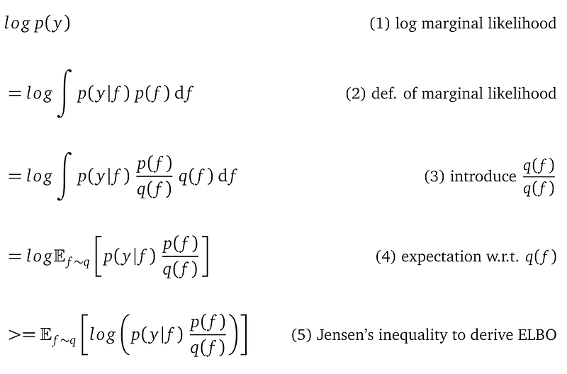
Line (1) is the notation for log marginal likelihood.

Line (2) expands the definition p(y) into an integration.

Line (3) introduces the quantity q(f)/q(f), which evaluates to 1. So this quantity does not change the result of the integration. This is a famous manipulation — it brings the variational distribution q(f) into the picture.

Line (4) re-writes the integration in line (3) into an expectation with respect to the random variable f from the variational distribution q(f).

Line (5) applies the Jensen’s inequality to move the log function from outside of the expectation to the inside of the expectation. The resulting expectation is the formula for ELBO. We use Jensen’s inequality to give us computation convenience — the expectation of a log is easier to manipulate than log of an expectation.

ELBO is a lower bound

Please note the change from the equal sign to the greater or equal sign after the application of Jensen’s inequality. It reveals that the ELBO is smaller than the log marginal likelihood log(p(y)) that we really wish to maximize. This marginal likelihood is also called model evidence. And our ELBO is lower than this evidence, hence the name Evidence Lower BOund.

You may ask, what is the difference between this ELBO lower bound and the log marginal likelihood log p(y) that we really want to maximize? We already know this difference from a previous equation:

The difference is the KL divergence between the variational distribution q(f) and the true posterior p(f|y). After rearranging some terms, we have:

Note that a KL divergence is a non-negative quantity, so KL(q(f)||p(f|y)) ≥0. This equation confirms that maximizing the ELBO is equivalent to minimizing the KL divergence between q(f) and p(f|y) because a larger ELBO means a smaller KL(q(f)||p(f|y)). To understand this point correctly, we need to go over some subtleties:

1. log(p(y)) is an expression that mentions the kernel parameters lengthscale l and the signal variance σ².
2. The ELBO is an expression that mentions the kernel parameters as well as the variational parameters μ and Σ.
3. The KL(q(f)||p(f|y)) is an expression that mentions the kernel parameters as well as the variational parameters μ and Σ.

Maximizing the ELBO by changing values of l, σ², μ, and Σ will change the value of log p(y) at the same time. You can’t treat log p(y) as a constant during the parameter learning process. But no matter which values the parameter learning process chooses for l, σ², once the ELBO is maximized in this model parameter value configuration, this very configuration gives you a minimized KL(q(f)||p(f|y)).

Analytical expression for the ELBO

Let’s see the ELBO formula again:

The ELBO is a function with the model parameters as arguments. We need to derive the analytical expression for the ELBO because we want to use gradient descent to find concrete values for those model parameters that maximize ELBO. Gradient descent only works for analytical functions because it computes gradients of that function with respect to its arguments.

The KL term is already analytical

Since both q(f) and p(f) are multivariate Gaussian probability density functions, the analytical form for their KL-divergence is known. This is one of the advantages of choosing q(f) to be a multivariate Gaussian. Later, I will show you the analytical expression for this KL term.

The likelihood term is not analytical

The likelihood term is an integration, so not analytical yet. Let’s manipulate it a bit:

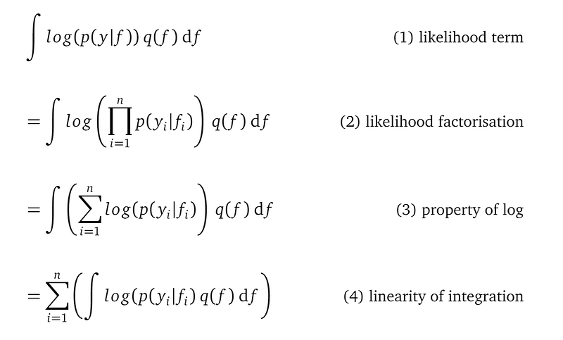
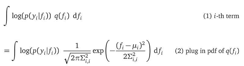
The above expression consists of n terms of the same structure. To derive the analytical expression for the whole likelihood term, we can focus on an arbitrary term, say the i-th term. The following is a very important derivation:

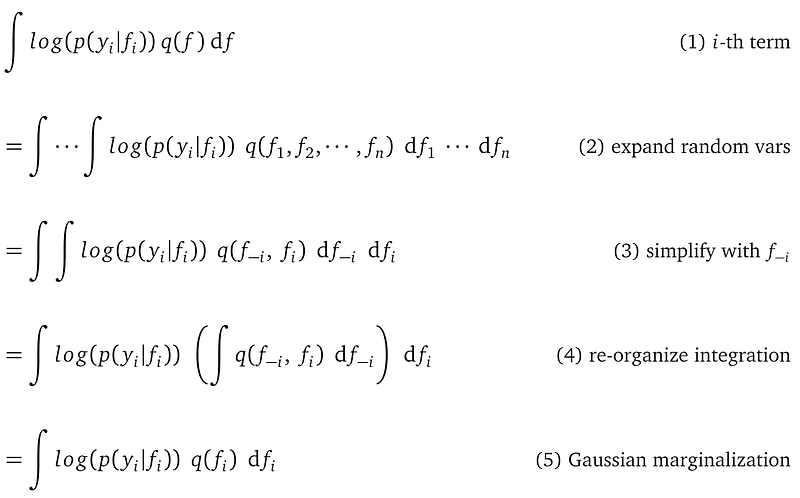
Line (1) is the formula for the i-th term inside the likelihood term. It is an n-dimensional integration over the random variable vector f. n is the number of training data points. This is because this integration is computing the expectation of log(p(yᵢ|fᵢ)) with respect to the variational distribution q(f), which is an n-dimensional multivariate Gaussian. Note log(p(yᵢ|fᵢ)) only mentions a single random variable in fᵢ, but q(f) mentions all n random variables.

Line (2) expands the random variable vector f into the individual random variables f₁ to fₙ. There are n random variables in f, so there are n single-dimensional integrations.

Line (3) introduces a name f₋ᵢ to represent the vector of random variables [f₁, f₂, … , fᵢ₋₁, fᵢ₊₁, …, fₙ]. This is a vector of length n-1. It contains all random variables in f except for fᵢ. We introduce f₋ᵢ to make the formulas shorter.

Line (4) re-groups the n integrations into 2 integrations: one over the single variable fᵢ, the other over the random variable vector f₋ᵢ. The reason is we want to apply the multivariate Gaussian marginalization rule to compute the inner integration over f₋ᵢ.

Line (5) applies the multivariate Gaussian marginalization rule to compute the inner integration over f₋ᵢ, leaving the result as q(fᵢ). Amazingly, we know the analytical expression for q(fᵢ). This step needs more explanation.

Recall q(f; μ, Σ) is a multivariate Gaussian distribution with mean vector μ and covariance matrix Σ. Here I show the entries of f, μ and Σ explicitly:

The above derivation at line (3) re-organizes the random variables in the distribution q into the fᵢ, f₋ᵢ blocks. At this line:

1. μᵢ is a float value; it is the mean value of the random variable fᵢ.
2. μ₋ᵢ is a float vector of length n-1; it is the mean values for the random variables in the vector f₋ᵢ.
3. Σᵢ,ᵢ² is a float value; it is the variance of the random variable fᵢ
4. Σᵢ,₋ᵢ² and Σ₋ᵢ,ᵢ² are matrices of size (n-1)×(n-1); they are transpose of each other. They represent the covariance between random variable f₋ᵢ and random variables in f₋ᵢ.
5. Σ₋ᵢ,₋ᵢ² is a matrix of size (n-1)×(n-1), is it the covariance among random variables in f₋ᵢ.

With the distribution of q reformulated this way, let’s go back to look at the inner integration over random variables f₋ᵢ:

This integration integrates out the random variables f₋ᵢ from the joint distribution q(fᵢ, f₋ᵢ), resulting in q(fᵢ), a distribution over a single random variable fᵢ. This is the meaning of marginalization in probability theory.

Since q(fᵢ, f₋ᵢ) is a multivariate Gaussian distribution, we can apply the multivariate Gaussian marginalization rule to trivially derive the analytical expression of q(fᵢ), which is equivalent to computing the above integration. This is the other advantage of choosing q(f) to be a multivariate Gaussian distribution.

The multivariate Gaussian marginalization rule says the marginalized distribution q(fᵢ) is still a Gaussian distribution, with mean and variance equal to the parts highlighted with red boxes in the joint distribution:

The highlighted part is a single-dimensional Gaussian distribution for the random variable fᵢ with mean μᵢ and variance Σᵢ,ᵢ². μᵢ is the i-th entry of the μ vector and is Σᵢ,ᵢ² is the i-th entry of the diagonal of the matrix Σ. The probability density function q(fᵢ) is:

With this, we can see that the i-th likelihood term is:

This is a function that only mentions a single μᵢ entry in μ and a single entry Σᵢ,ᵢ² in Σ. Generalizing to all the likelihood terms, we know the overall likelihood mentions all entries in the vector μ and only the diagonal entries of Σ.

Which model parameters does the likelihood term mention?

Importantly, only the variational parameter μ and the diagonal entries in the variational parameter Σ are mentioned in the likelihood term. The off-diagonal entries in Σ are not mentioned in the likelihood term. The kernel parameter l and σ² are not mentioned in the likelihood term either.

The likelihood is the sum over n single-dimensional integrations

The above formula reveals that the i-th likelihood term is a one-dimensional integration over a single random variable fᵢ. Generalizing to arbitrary terms in the likelihood, we know they are all single-dimensional integrations, with each integration over a different random variable in f.

So if we can work out the analytical expression representing the result of the integration in the i-th likelihood term, we will be able to work out the analytical expression for the whole likelihood. With the KL term already being analytical, we will have the analytical expression for the whole ELBO. This will enable us to use gradient descent for parameter learning.

The fact that the i-th likelihood term is a single dimension integration is very important. Because this likelihood term is an integration. As we said before, it is an operation, not an analytical expression that we can evaluate. This single-dimensional integration is hard to compute as well. But since it is one dimensional, we can apply a method, called Gaussian quadrature, to approximate the result of this integration in an analytical way.

Gaussian quadrature

The Gaussian quadrature rule, or more specifically, the Gauss-Hermite quadrature rule, shown below, says that the result of the integration of the particular structure on the left-hand side can be approximated by the sum of m terms on the right-hand side, with F(t) being a function of t:

On the right-hand side, wⱼ and tⱼ are pre-computed and we can look them up from a Gaussian quadrature table. And F(tⱼ) is the evaluations of the function F at locations tⱼ. The right-hand side is an analytical expression because we can look up wⱼ and tⱼ and we can evaluate F(tⱼ). Both the left- and the right-hand side evaluates to a number.

Please distinguish between the two approximations that we introduced:

1. Previously we introduced the variational distribution q(f) to approximate the true posterior p(f|y). The way we force q(f) to get close to p(f|y) is to maximize the ELBO. This is a distribution to distribution approximation.
2. Now we need to derive the analytical expression for the i-th likelihood term in the ELBO. Since the integration is difficult to compute, we want to use Gaussian quadrature to approximate the result of this integration. This is a number to number approximation.

For now, please accept that the Gaussian quadrature approximation makes sense. In fact, this approximation is usually very close to the true result of the integration. In this sense, the Gaussian quadrature approximation is an estimator of the true integration value. Since the approximation is not the same as the integration result, this estimator has a bias, measured by the difference between the approximation and the true integration result. And the bias can be arbitrarily small if you choose a large enough m, at the expense of more computation.

Intuitions behind Gaussian quadrature

I will write another article to explain why Gaussian quadrature makes sense. But to calm your curious mind down for now, here is a simple explanation.

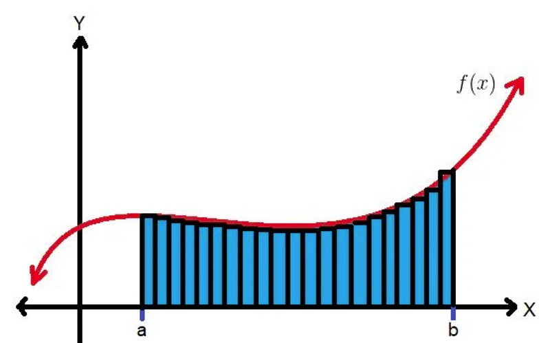
You can understand the result of an integration as a sum over infinitely many rectangles with equal width, as the following figure illustrates. Each rectangle has an infinite small width and its height is the value of the integrand at the x-location of that rectangle.

We can approximate the result of the integration by carefully selecting only a few (instead of infinitely many) rectangles at different x-locations, and give these rectangles different widths. In areas where the function moves slowly, the rectangles are wider, in areas where the function moves rapidly, the rectangles are narrower. The following figure illustrates this idea.

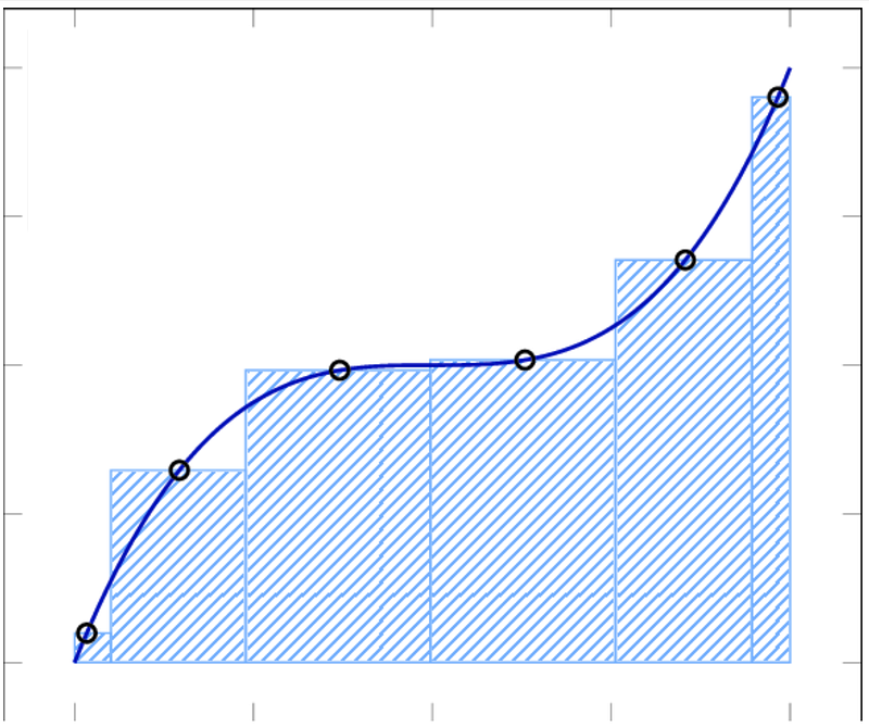
The weighted sum structure in the Gaussian quadrature formula implements exactly the above idea. The quadrature theory tells you how to choose the location tⱼ to evaluate the integrand and what the width wⱼ should this rectangle has. Those locations and widths are already calculated for you in a table. You only need to decide how many rectangles you want, that is the m value. The more rectangles you want, the more precise the approximation, but the more expensive the calculation.

Amazing, isn’t it?

Using Gaussian quadrature to approximate the i-th likelihood term

Now, let’s use Gaussian quadrature to develop the analytical expression that approximates the result of the i-th likelihood term.

Looking at the integration again:

This is not of the format required by the left-hand size of the Gaussian quadrature rule:

We need to transform this integration into the format required by the Gaussian quadrature rule. Quite often, the things we do in math is pattern matching.

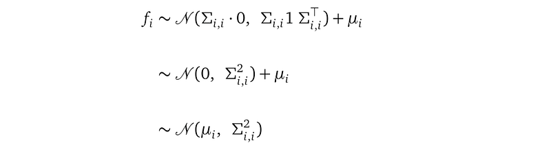
Since the integration in the i-th likelihood term is an expectation with respect to a Gaussian random variable fᵢ ~ 𝒩(μᵢ, Σᵢ,ᵢ²), let’s first apply the rule of change-of-variable in integration to turn it into an expectation with respect to a standard Gaussian distribution 𝒩(0, 1). We introduce a new one-dimensional random variable u coming from a standard Gaussian distribution: u~𝒩(0, 1).

We can define the random variable fᵢ as:

Using the Gaussian linear transformation rule, it is easy to verify that fᵢ defined in this new way still comes from the distribution 𝒩(μᵢ, Σᵢ,ᵢ²):

You can see my other article Demystifying Tensorflow Time Series: Local Linear Trend to find more about the Gaussian linear transformation rule.

With this new random variable u, we transform the i-th likelihood term as:

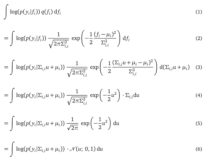
Line (2) expands the probability density function for fᵢ.

Line (3) applies the change-of-variable rule to change the integration variable from fᵢ to u.

Line (4) and (5) simplifies the formula. At line (5), the probability density function of a standard Gaussian distribution pops out.

Line (6) recognizes that now the i-th likelihood term is an expectation with respect to a standard Gaussian random variable u.

We realize that the formula at line (5) is still not the format we need to apply Gaussian quadrature. But the desirable format is just another change-of-variable away. We introduce a new variable t:

And transform the i-th likelihood term as:

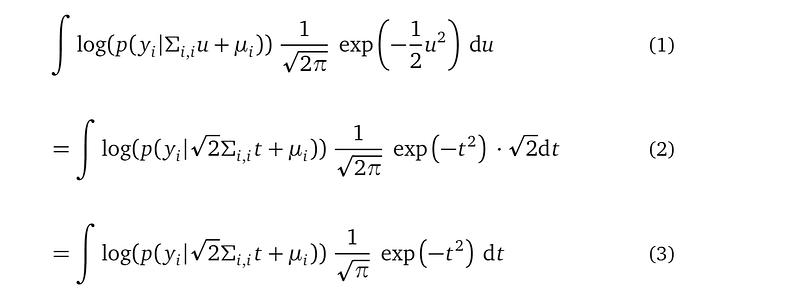
We finally transformed the i-th likelihood term into the format required by the Gaussian quadrature rule, with:

In these two applications of change-of-variable, all the old and new variables fᵢ, u, and t, have domain from -∞ to +∞, so these operations do not change the boundary of the integration — so we ignored the boundaries all together.

By applying the Gaussian quadrature formula that we’ve been wanting for so long, we can derive:

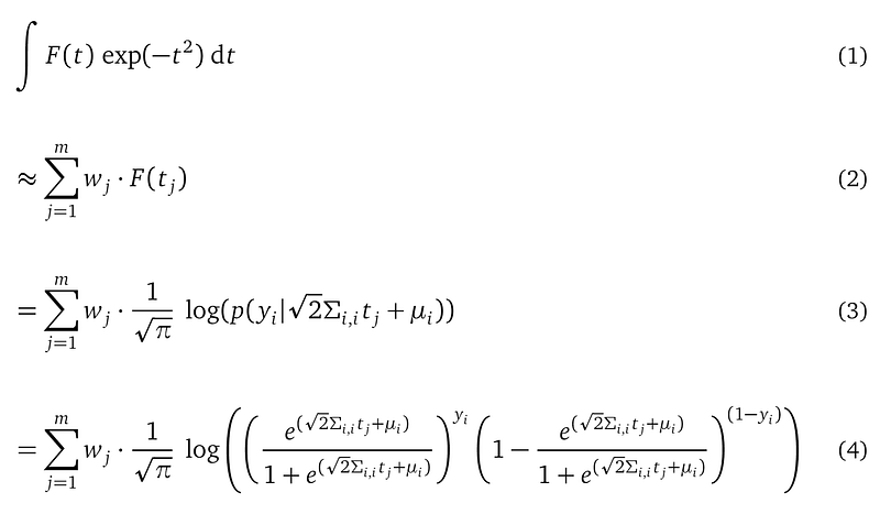
Line (1) and (2) are the Gaussian quadrature formula.

Line (3) plugs in F(t).

Line (4) writes out everything in the likelihood. Let’s read it carefully because it reveals important information:

1. This formula is analytical because we can evaluate its value after we plug Yᵢ into yᵢ, decide on the value m, and replace all wⱼ and tⱼ with values from Gaussian quadrature table. It evaluates to a single real value.
2. Since each i-th likelihood term consists of m terms, the entire likelihood term consists of m×n terms, with n being the number of training data points. This seems to be a lot of terms, for example, if m is 40 and the number of training points is 1000, we have 40,000 terms for the likelihood term. But it is affordable because the number of terms scales linearly with n, with a constant scaling factor m. Anything that scales linearly is good news for Gaussian Process.
3. This expression is a function that mentions the variational parameter μ and the diagonal entries from Σ. Since this expression is part of the ELBO, which is our objective function to maximize, it does satisfy our requirement for an objective function — it needs to mention at least some of our model parameters. The likelihood term in ELBO only mentions part of variational parameters, and it does not mention the kernel parameters from the GP prior. Please remember this, and we will detail it a bit later.

Constant in the quadrature formula

To give you some taste of the Gaussian quadrature table, when we choose m=10, the values of location tⱼ and weight wⱼ are:

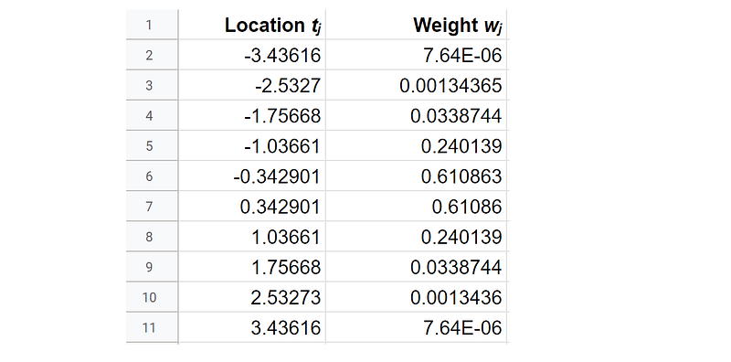
The more terms you use (the larger m), the more precise the approximation, but the more expensive the computation is. A rule of thumb is to use m=40.

Congratulations! We derived the analytical expression for the whole ELBO, we are ready for parameter learning. Before doing that, a responsible machine learning practitioner would ask a few questions.

Is Gaussian quadrature a good approximation?

Since we are using Gaussian quadrature to give us an analytical expression to approximate the result of the integration in the i-th likelihood term, we need to know how good this approximation is and how computationally affordable it is.

Gaussian quadrature is very precise. You can look at the video The Magic of Gaussian Quadrature — A Billion Times Better than the Next Best Thing to convince yourself. In fact, the bias of Gaussian quadrature is negligible. There is little difference between the Gaussian quadrature approximated result from the true value of the integration.

Gaussian quadrature is a deterministic procedure, there is no variance in the approximation — you call the Gaussian quadrature method any number of times, you get the same result.

So Gaussian quadrature is a good approximation to the i-th likelihood term.

Why all model parameters can be learned from training data?

We saw that the analytical expression of the i-th likelihood term only mentions the variational parameters μ and only the entries in the diagonal of the other variational parameter Σ. It does not mention the kernel parameters l and σ² either, which are from the GP prior.

Also, we notice in ELBO, only the likelihood term mentions the training data Y. You may ask, how can the off-diagonal entries of Σ and the kernel parameters l and σ² be learned from data? This is a very important question. A connection between our training data to all the model parameters is a necessary condition such that these model parameters can be learned from training data by gradient descent.

To answer this question, we need to investigate the analytical expression of the other term in ELBO, the KL divergence term between the variational distribution q(f; μ, Σ) and the prior p(f; l, σ²).

The first thing to notice is the matrix inversion K⁻¹, with K being the covariance matrix from the GP prior. The shape of K is n×n, with n being the number of training data points. So this inversion is very expensive. This also means, our model cannot scale to large datasets.

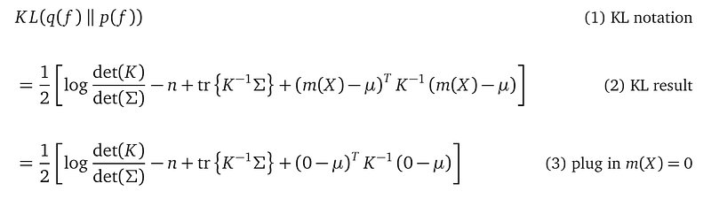
Line (2) gives the analytical expression for the result of the KL divergence between q(f; μ, Σ) and p(f; l, σ²). Both are multivariate Gaussian distributions over the same random variables f. The computation is a bit complicated, please just accept that this can be done and it is analytical. n is the number of training data points. tr stands for the trace operator, which is the sum over the entries in the diagonal of a square matrix. K is the n×n covariance matrix defined in the GP prior. det(K) stands for the determinant of K. K⁻¹ is the inverse of K. And m(X) is the mean function we give to the GP prior, usually, m(X)=0.

Line (3) plugs in the zero mean function 0 into the formula to simplify it.

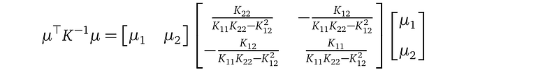
Let’s investigate the formula at line (3) with a two training data point (X₁, Y₁), (X₂, Y₂) example:

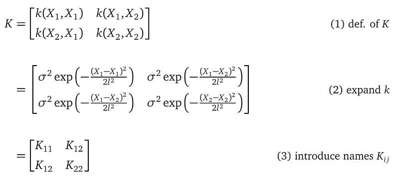
The covariance matrix K only mentions X in the training data, and not Y. And K, being a covariance matrix, is symmetric. And K mentions the kernel parameters l and σ².

Let’s look at our variational distribution (here, I write an entry of the covariance matrix as Σᵢⱼ to save space, instead of the notation Σᵢ,ⱼ² which I used before:

With the above definitions, we can compute the determinant det(K), det(Σ), and the inverse K⁻¹ using rules from calculus:

Now, we can write down the terms inside the KL divergence formula:

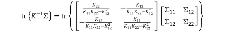
We only need to glimpse at these terms to see that in the KL divergence term:

1. All model parameters, including all entries in μ and all entries (diagonal, as well as off-diagonal) in Σ from the variational distribution, and l and σ² from the GP prior, are entangled together.
2. Because of this entanglement, the part of the model parameters mentioned in the likelihood term (i.e., μ and diagonal entries of Σ) can impact the rest of the model parameters that are not mentioned in the likelihood term (off-diagonal entries of Σ, and l and σ² from the GP prior).
3. And transitively, the training data Y can impact all model parameters.

This is why all the model parameters can be learned from the training data.

Model scalability

The matrix inversion K⁻¹ in the KL divergence from q(f) to p(f) is expensive to compute. The number of operations, such as multiple or add two numbers in the matrix, scales with n³. n is the number of training data points. For n=1000, a tiny data set in the modern standard, the inversion requires billions of operations.

This means our variational Gaussian process cannot scale to large data sets — it just takes too long to compute K⁻¹. My next article will be on the Sparse And Variational Gaussian Process, a model that can scale to large datasets.

Can we use Gaussian quadrature to compute the posterior?

You may ask, we used Gaussian quadrature to approximate the likelihood term in ELBO, can we use it to approximate the marginal likelihood in Bayes rule?

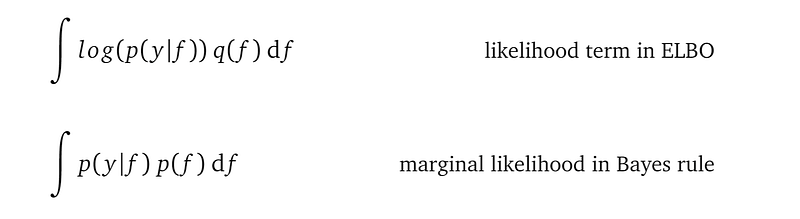
The variational distribution q(f) and the GP prior are both multivariate Gaussian distributions. So structurally, these two integrations are the same. Why don’t we use Gaussian quadrature to approximate marginal likelihood? I totally relate to this question — it drove me crazy as well.

But there is a crucial difference between log(p(y|f)) in the ELBO likelihood term and the p(f|y) in the marginal likelihood. The marginal likelihood does not have a log in front. So we cannot use the property log(ab) = log(a) + log(b) to decompose the marginal likelihood into a sum of smaller terms. Without this, we cannot apply the multivariate Gaussian marginalization rule to the marginal likelihood to reduce the n-dimensional integration over f to a sum of single integrations over single random variable fᵢ.

As a result, the marginal likelihood remains an n-dimensional integration, and the Gaussian quadrature approximation for it requires mⁿ terms, that’s m to the power of n terms — the number of total terms grows exceptionally with the number of training data points. This is an unpractically large number for even a small data set. This is the reason why we cannot afford to use Gaussian quadrature in the direct calculation of the posterior.

The appendix of this article shows you why Gaussian quadrature requires mⁿ terms to approximate the marginal likelihood.

Parameter learning

Now we have derived the analytical expression for the ELBO. This expression is a function with all our model parameters as unknowns — the kernel parameter l, σ², and the variational parameters 𝜇, Σ. Parameter learning uses gradient descent to maximize the ELBO to find optimal values for these model parameters. It is a straightforward application of gradient descent. But thinking carefully about this optimization raises some interesting questions.

Let’s first summarize our model.

The full model

Our binary classification model has the following components:

1. The multivariant Gaussian prior p(f; l, σ²), which introduces the latent random variable vector f, and the kernel parameters l and σ².
2. The Bernoulli likelihood p(y|f), which introduces the observational random variable vector y, and does not introduce any parameter.
3. The variational distribution q(f; μ, Σ), which introduces the variational parameters μ and Σ. We require q(f; μ, Σ) to be close to the posterior p(y|f; l, σ²) in the KL-divergence sense.

In math language, the model reads (model parameters in red):

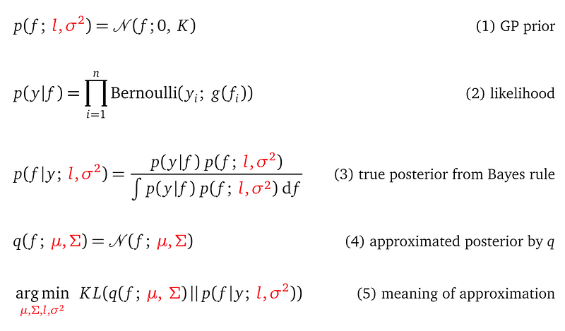
Line (1) is the GP prior. Line (2) is the likelihood. Line (3) defines the true, but intractable, posterior computed by Bayes rule. Line (4) introduces the variational distribution to approximate the true posterior. Line (5) uses the KL divergence to define the meaning of approximating the true posterior by the variational distribution. This KL divergence is intractable as well, so we ultimately maximize the ELBO as a proxy for minimizing this KL.

How many scalars do we need to learn?

Our model has four parameters of different shapes (shape in the sense of the shape of a tensor):

• The lengthscale l is a scalar.
• The signal variance σ² is also a scalar.
• q(f)’s mean vector μ is a vector of length n, so it has n scalar entries.
• q(f)’s covariance matrix Σ is a matrix of size n×n, and it is symmetric, so has ½n(n+1) free scalar entries.

In total, this model has 2+n+½n(n+1) scalars whose values need to be decided by parameter learning. Don’t overlook the task of listing all the model parameters — this is a sanity check so you understand the model.

I know that you want to shout out: 2+n+½n(n+1) is a lot of scalars, it is more than the number of training data points n!

Since most of the scalars come from the parameters of the variational distribution q, can we parameterize q with fewer scalars? Yes, that is the mean-field parameterization.

Mean-field parameterization for q

Our variational distribution q(f; μ, Σ) is a full multivariate Gaussian distribution because Σ is a full covariance matrix with no zeros. if we require Σ to be a diagonal matrix, then q(f) becomes a mean-field distribution.

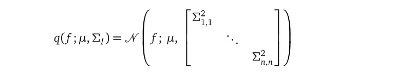
The motivation of using a mean-field q(f) is that there are fewer variational parameters to learn. Instead ½n(n+1) free scalars from a full covariance matrix, we now only have n free scalars from the diagonal of the mean-field covariance matrix because it is a diagonal square matrix. The total number of scalars that we need to learn in a mean-field configuration is 2+2n. The parameter learning process is easier with fewer model parameters, meaning the optimization stops quicker.

The downside of this mean-field approximation is that it can only model a much smaller subset of distributions — the ones that constraints all the random variables to be independent of each other. However, in reality, the random variables in a true posterior often correlate to each other. This means the mean-field approximation is a more coarse approximation compared to the variational distribution with a full covariance matrix.

This is the trade-off between model capacity and computational cost that we have to decide. A common practice is to start with a mean-field approximation. If the learned model does not perform well in prediction, move to a more expensive, full covariance approximation.

When the variational distribution q(f; μ, Σ) has a mean-field structure, i.e., Σ is a diagonal matrix, all individual random variables in f are independent of each other — there's no relationship among any two of them. So information about one individual random variable, say fᵢ cannot be used to reason about another individual random variable, say fⱼ. You may wonder how our model can make predictions.

Our model can make predictions at a testing location X_* because even though the correlations among random variables in f, which are at training locations X, are zero, the correlation between f and the random variables f_* at testing location X_* is not zero. This non-zero correlation is the conditional probability p(f_*|f) that we impose through the prior. It enables the model to reason about the values of f_* by using information from f. We will see this more clearly in the Making predictions section.

A model with too many parameters?

After counting the number of scalars that we need to learn, we realized a problem — our model has more scalars (2+n+½n(n+1) in the full Gaussian configuration and 2+2n in the mean-field configuration) to learn than the number of training data points, which is n.

This is bad because the model now has the capacity to fit the training data exactly — the model can just use its parameters to remember where the training data is. But this model is not able to generalize to new data. People use the term overfit to refer to this situation of model fits the training data arbitrarily well but make bad predictions on testing data.

By the way, the model having enough parameters to fit the training data arbitrarily well does not mean gradient descent can find concrete values for those parameters to fit the training data well. The more parameters a model has, the harder it is for gradient descent to navigate through the parameter value space. It is possible that gradient descent converges to some model parameter values that do not even fit the training data well.

Ideally, we want a model to have just a sufficient number of parameters and sufficient model structure (the kernel function, the likelihood function, etc.) such that the model can summarize the underlying characteristics of the training data well, instead of remembering where the training data is. This summarization also gives the model the ability to generalize to new, testing data. But by design, our binary classification model, with too many parameters, is not a good model. What a bummer.

In fact, the real reason for you to learn about this model is to familiarize you with how to apply variational inference to a Gaussian Process model. This is to get you ready for the actual practical model — the Sparse and Variational Gaussian Process model (SVGP model). You can read more about the SVGP model at: Sparse and Variational Gaussian Process — What To Do When Data is Large later. For now I suggest you finish this article first.

No stochastic gradient descent?

The ELBO consists of the likelihood term and the KL term. Both terms require full data to evaluate. The likelihood term, shown below, requires the full Y.

And the KL term, shown below, requires all the training data to compute:

The formula at line (3) mentions the covariance matrix K=k(X, X) from the prior. K needs the whole X to compute.

So at each optimization step, the gradient descent algorithm needs to go over all the training data to compute the ELBO as well as its gradient. This is why we cannot use stochastic gradient descent on our variational model. Stochastic gradient descent only uses a batch of the training data on each optimization step, so it requires much less memory, and often it converges much faster.

The good news is that the Sparse and Variational Gaussian Process model that I will talk about in my next article can utilize stochastic gradient descent. So stay tuned, everything will eventually work out.

Too much pressure on gradient descent?

We use gradient descent to maximize the objective function ELBO. If we think carefully, the ELBO actually encodes two optimizations in one single formula:

1. Find values for the kernel parameters l and σ² such that the true posterior explains the training data well.
2. Find values for the variational parameters μ, Σ such that the variational distribution q(f; μ, Σ) closely approximates the true posterior.

That’s a lot to ask from gradient descent. What this means mathematically is: the ELBO can be highly non-concave with a lot of local maximas. Gradient descent, being a local optimization method, will get stuck on one local maxima, and not necessarily a good one. So how do we optimize such models becomes its own art/science:

• which optimizers to use?
• how do we decay the learning rate?
• how do we initialize the model parameters before optimization starts?
• how do we handle numerical instability? For Gaussian Process models, this means Cholesky decomposition failure when we inverse a matrix.

This is a big topic, and I will dedicate a couple of articles in a short future to explain it.

Making predictions

Now we have the posterior p(f|y ) for the random variable f, which is at training locations X. In fact, we don’t have p(f|y). We have the variational distribution q(f) that behaves similarly to our posterior. But let’s keep using p(f|y) as if we know it.

Using posterior to make predictions

Let’s first make it clear why we need the posterior to make predictions.

Our full model consists of three random variables, f_*, f, and y. f_* and f are latent random variables, they don’t have corresponding observations. y is an observational random variable, it has observations Y from our training data.

Through the GP prior p(f_*, f) we imposed some characteristics over the random variables f and f_*. Through the likelihood p(y|f), we established the connection between the latent random variable f and the observational random variable y.

The Bayes rule uses the observations Y to give us updated characteristics of f and f_* in the form of the posterior distribution p(f_*, f|y). This is the reason why we want to use the posterior to make predictions — the posterior re-weighs all functions in the prior such that functions that explain the training data better receive higher probabilities.

The posterior p(f_*, f|y) is a distribution over random variable f_* and f. But we only need to make predictions for f_*, in other words, we only need a distribution over f_*. So we integrate our the random variable f from p(f_*, f|y) to result in the predictive distribution p(f_*|y).

Note even our model consists of three random variables f_*, f and y. We don’t have to know the joint probability density, denoted as p(f_*, f, y), over them three. Throughout this article, this joint distribution p(f_*, f, y) never appeared. We can compute what we need, which is the predictive distribution p(f_*|y), without needing p(f_*, f, y). This is a good thing because p(f_*, f, y) = p(f_*, f|y) p(y) and we know the marginal likelihood p(y) is not an easy quantity to work with. We defined our model in the way it is defined to make sure that we don’t have to touch the joint distribution p(f_*, f, y).

Posterior in the form of Gaussian distribution

To make predictions at testing locations X_*, we need to derive the posterior p(f_*|y) for the random variable f_*, which are at testing locations.

Line (2) uses the chain rule in probability theory in reverse to split the joint distribution.

Line (3) drops y under the condition of p(f_*|f, y). We can do this because the GP prior only mentions f and f_*. So given f, f_* is independent of y. y is introduced in the likelihood.

Line (4) replaces the posterior p(f|y) that we don’t know by our variational distribution q(f), which we know. This is an important step:

• q(f) has the same API as the posterior p(f|y). And,
• it behaves similarly to the posterior, in the minimum KL divergence sense.

So we can replace p(f|y) with q(f), that’s the whole point of variational inference.

At line(5), inside the integration sign, p(f_*)|f) is the conditional distribution derived by applying the multivariate Gaussian conditional rule (here for more details of this rule) on the GP prior:

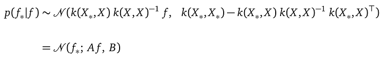
And we introduce the name A and B to shorten the formula, with:

A and B mentions both the training location X and the testing location X_*. They establish the connection from f to f_*.

Line (6) applies the multivariate Gaussian linear transformation rule to write the distribution of the random variable f_* by using only the mean μ and covariance matrix Σ of f from q(f; μ, Σ) without mentioning f.

Line (7) moves the probability density function for f_* outside of the integration since it does not mention the integration variable f, so it can be treated as a constant with respect to the integration.

Line (8) computes the integration to 1 since the integration of a probability density function over the domain of the random variables evaluates to 1.

The result is the posterior distribution p(f_*|y) for random variables f_* at testing locations X_*. We also call it the predictive distribution. It is a single-dimensional Gaussian distribution if f_* is single-dimensional, and it is a multivariate Gaussian distribution if f_* is multi-dimensional.

The predictive distribution

The full formula for the predictive distribution, with A and B expanded, is:

with:

A few important things to notice:

First, the predictive distribution does not mention the training data Y. You may still remember in a Gaussian Process regression model (Computing the posterior section), the mean of the predictive distribution is a weighted sum of the training data Y. But in our variational model, the mean of the predictive distribution is a weighted sum of the mean μ from the variational distribution q. The information of Y is completed absorbed into the value of μ during the parameter learning process.

Second, the predictive distribution mentions the training data X — you see X all over the place in both the mean and the variance of the predictive distribution. This is because the model needs to use the distance between the training location X and the testing location X_* to compute the correlation between the variable f(X) and f(X_*) — the farther the distance between X and X_*, the smaller the correlation, and the less weight the model gives f(X) to predict the value of f(X_*).

Finally, we understand how our model can make predictions even the variational distribution q has a mean-field structure, in which case, Σ is a diagonal matrix. Our model uses the correlation k(X_*, X) matrix to link the random variables f at training locations X and the random variables f_* at testing locations X_* together. The correlation k(X_*, X) is introduced through the conditional probability p(f_*|f); it does not care whether the individual random variables in f are independent of each other.

Posterior in the form of Bernoulli distribution

In the binary classification setting, we need to make predictions in the form of Bernoulli distribution, not in the form of a Gaussian distribution.

To construct the Bernoulli posterior, we need to decide the value of its single parameter:

Let’s assume there is a single testing point, so X_* is a scalar, instead of a vector. So f_* is a one-dimensional Gaussian random variable from our posterior p(f_*|y). Defined this way, g(f_*) is a random variable, but a Bernoulli distribution needs a scalar for its parameter, so we compute the expected value for g(f_*) with respect to f_*:

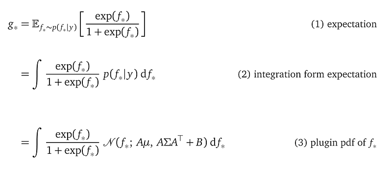
You will happily realize line (3) is an integration that you can use Gaussian quadrature to approximate.

With g_* computed, the Bernoulli probability density for y_* is:

or equivalently:

The above Bernoulli probability density function is our final prediction for a testing location. You may ask, shouldn’t all predictions from a Gaussian Process model come with an uncertainty measure? Yes, and the Bernoulli distribution does have its uncertainty measure, inherited from the Gaussian posterior. Since the Bernoulli distribution is a discrete distribution, it’s uncertainty is encoded in the probability parameter g_*:

• g_* close to 1: the model is certain about the event y_*=1.
• g_* close to 0: the model is certain about the event y_*=0.
• g_* close to 0.5: the model is uncertain about which label to predict.

Remember g_* is a derived quantity. It gets its value from the posterior p(f_*|y). The mean and variance of p(f_*|y) are the two things (together with the test location X_*) that determine the value of g_*. Hence, they determine the uncertainty of the Bernoulli prediction.

Experiment result

I used this code to create a variational Gaussian Process model. It uses gpflow, a Python library for Gaussian Process models.

The following figure shows what the model predicts for our training data (X, Y) after parameter learning.

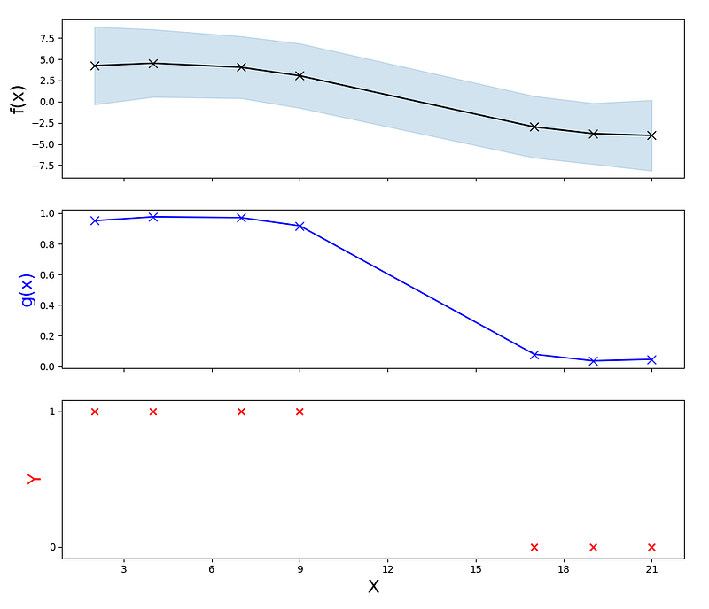
The top subplot shows the predictions from the Gaussian posterior f(x)=p(f|y). The predictions are in the form of mean and variance. So the top subplot shows the mean in black and the 95% confidence interval in cyan. You can see that for data points with label 1, f(x) values are around 4, and for data points with label 0, f(x) values are around -4.

The middle subplot shows the squashing function g(x) in blue. We can see that it evaluates to values close to 1 for data points with label 1, and evaluates to values close to 0 for data points with label 0.

The bottom subplot shows our training data in red.

This plot is very similar to the hand-drawn plot at the beginning of this article.

Conclusion

Here I summarize the main steps in our Variational Gaussian Process model:

1. The model uses a multivariate Gaussian prior p(f), and it uses a Bernoulli likelihood p(y|f) to model binary observations.
2. When the likelihood is non-Gaussian, the Bayes rule results in an intractable posterior p(f|y).
3. A variational distribution q(f) is used to approximate the posterior p(f|y). And we define a good approximation by requiring the KL-divergence KL(q(f)||p(f|y)) to be minimal.
4. The formula for KL(q(f)||p(f|y)) is also intractable. So we used the ELBO formula as a proxy to the KL(q(f)||p(f|y)) minimization task. We need to maximize the ELBO. The ELBO formula is tractable. We need to derive the analytical expression for the ELBO, which is an expression that mentions all the model parameters. This way, we can use gradient descent to maximize the ELBO with respect to the model parameters to find concrete values for those model parameters.
5. The ELBO consists of two terms, the likelihood term, and a KL term KL(q(f)||p(f)). The KL term is already analytical. But the likelihood term is an integration that is hard to compute.
6. The likelihood term, which is an n-dimensional integration, can be decomposed into n single-dimensional integrations. Gaussian quadrature provides an analytical approximation for the result of each of these single-dimensional integrations.
7. Gradient descent maximizes the analytical expression for the ELBO to find concrete model parameter values.
8. Finally, we point out that our model contains more parameters than the number of training data points. This is not a practical model. It serves as a preparation for the real practical model that we will learn next — the Sparse and Variational Gaussian Process model.

Support me

If you like my story, I will be grateful if you consider supporting me by becoming a Medium member via this link: https://jasonweiyi.medium.com/membership.

I will keep writing these stories.

References

The Variational Gaussian Process

Appendix: can we use Gaussian quadrature to approximate the marginal likelihood?

Here I give the derivations showing that the Gaussian quadrature approximation for the marginal likelihood from the Bayes rule requires mⁿ terms. The goal is to convince you that it is not practical to use Gaussian quadrature to approximate the marginal likelihood term. I suggest you go through these derivations because they are very good Bayesian statistics practices.

Here is the Bayes rule again:

As we said before, we can not use this rule to compute the posterior because the integration in the denominator is intractable. Now let’s try to use Gaussian quadrature to approximate this integration.

The likelihood p(y|f) is a product of n Bernoulli probability density functions, as we derived before and shown again here:

Since there is no log in front of p(y|f), we cannot use the property of log to decompose the likelihood into the sum of n log Bernoulli probability density functions, each for a single data point. This will cause the Gaussian quadrature rule to result in an exponential number of terms. To understand why, let’s continue our analysis.

Let’s manipulate this integration by applying the change-of-variable rule:

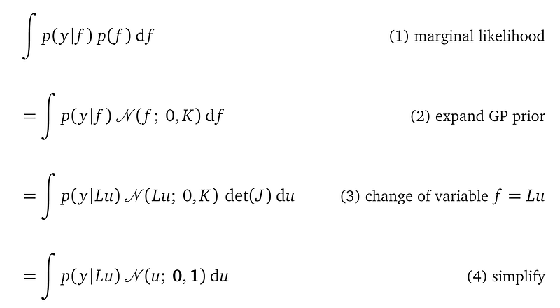
Line (1) is the integration in the denominator that we want to derive the analytical expression for. The integrand is the Bernoulli likelihood p(y|f) times the GP prior p(f).

Line (2) writes out the distribution of the GP prior, which is a multivariate Gaussian distribution with 0 mean and covariance matrix K.

Line (3) applies the change-of-variable rule in integration, by introducing the new variable u and rewriting the original integration variable f as Lu, where L is the lower triangular matrix of the Cholesky decomposition of the covariance matrix K. And u is an n-dimensional standard Gaussian distribution with 0 mean and identity covariance matrix 1. 0 is a 0 vector of length n, and 1 is an identity matrix of shape n×n.

Line (4) simplifies line (3). We need more explanation on how to derive this simplification, but first, we verify that f redefined as Lu still comes from the same Gaussian distribution 𝒩(0, K). Since f is a linear transformation from u, we use the Gaussian linear transformation rule to write the distribution of f from the distribution of u, which is a multi-dimension standard normal distribution 𝒩(0, 1).

For more details about the Gaussian linear transformation rule, please see Demystifying Tensorflow Time Series: Local Linear Trend, and search for “linear transformation”.

Now we have verified that f is still coming from the GP prior. To show how we arrived at the integration at line (4) above, let’s use an example with 3 data points. So

expands to:

To apply the change-of-variable integration rule, we need to compute the Jacobian matrix, and then compute the determinant for the Jacobian matrix:

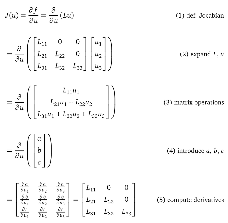
All the above derivations are simple. At line (4) introduces name a, b, and c to shorten the formula so everything stays in one line.

This derivation shows that the Jacobian matrix is equal to the lower triangular matrix L from Cholesky decomposition. So det(J(u)) = det(L).

Now let’s see the effect of the change-of-variable f=Lu on the GP prior p(f):

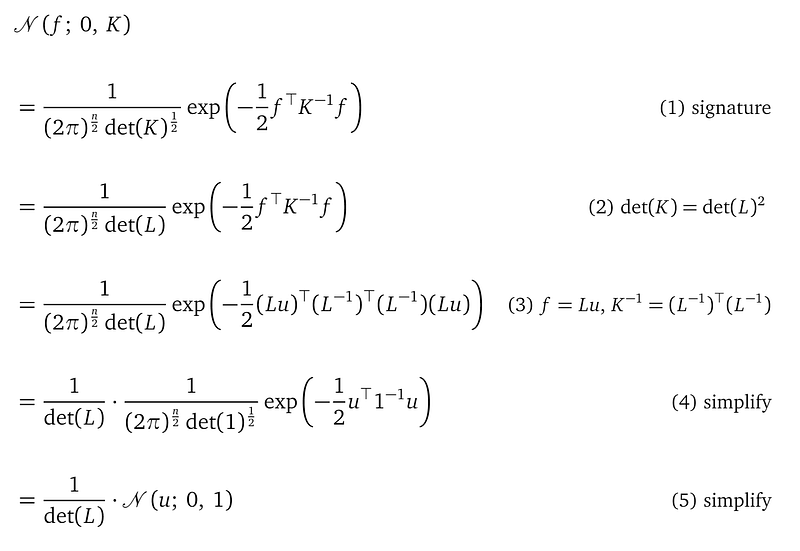
Line (2) uses the property det(K) = det(L)². This is a nice property are from the Cholesky decomposition.

Line (3) plugs in f=Lu and uses the property, also from Cholesky decomposition:

Line (4) simplifies the formula. It moves det(L) out of the original denominator and added the square root of det(1), which equals to 1. This is because we want to construct the formula of the unit multivariate Gaussian.

Line (5) recognizes that the formula equals to the probability density of u, scaled by 1/det(L). And we will happily realize that 1/det(L) cancels the det(L) coming from det(J(u)).

Before we conclude this change-of-variable derivation, we need to verify the integration boundaries before and after the change-of-variable operation.

The original integration has f as its integrated variable. f is a vector of Gaussian random variables. So each random variable in f has a domain of the full real line. After we applied the rule of change of variables, the integration variables become u, which is also a multivariate Gaussian random variable with the full real domain. That’s why we are implicit about the boundaries in the derivations.

Using Gaussian quadrature

Now we have the following integration, and we want to use Gaussian quadrature to give us the analytical expression that approximates its result:

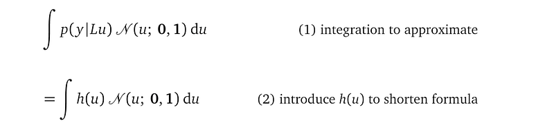
Line (1) is the integration to approximate. Line (2) introduces name h(u) = p(y|Lu) to shorten the formula for following derivations.

In our 3 data point example, u is a 3-dimensional standard normal distribution, so the above is a 3-dimensional integration. But the Gaussian quadrature rule only applies to single dimensional integration.

The nice thing about the standard multivariate Gaussian 𝒩(u; 0, 1) is that all the individual random variables u₁, u₂, u₃ are independent to each other because of the identity covariance matrix 1. So the joint distribution 𝒩(u; 0, 1) decomposes into:

With this decomposition, we have:

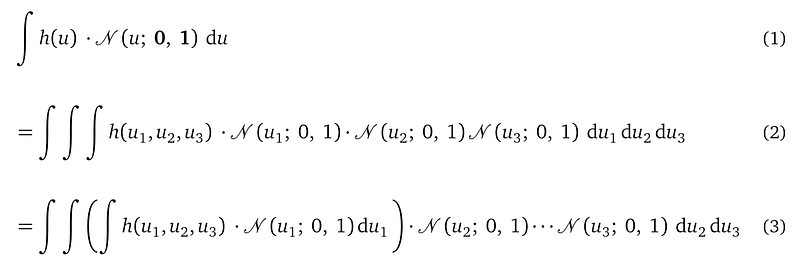
Line (2) expands u into individual random variables and their probability density functions. The likelihood h(u₁, u₂, u₃) is a function of all three random variables.

Line (3) groups the integration with respect to the random variable u₁ into a pair of parenthesis. Because we will be solving this innermost integration first.

And here it is:

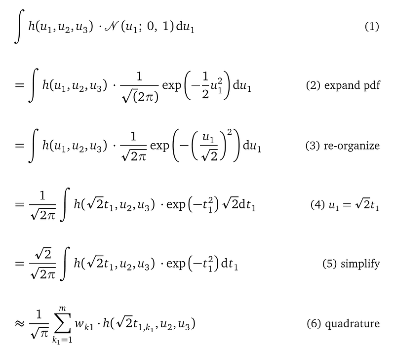
Line (2) expands the probability density function for 𝒩(u₁; 0, 1).

Line (3) re-organizes terms inside the exponential function to prepare for the change of variable in the next line.

Line (4) applies the rule of change of variable in integration, with the new variable t₁ such that u₁=√2 t₁.

Line (5) simplifies the formula into a form that we can apply the Gaussian quadrature rule.

Line (6) applies the Gaussian quadrature rule to approximate the integration with m terms.

The reason for the exponential number of terms

Notice at line (6) that even though the random variable u₁ has been “integrated” out by Gaussian quadrature, the function h still contains random variables u₂ and u₃. That’s where the exponential number of terms is coming from. Because now we have to apply the Gaussian quadrature rule, again and again, to integrate out the random variables one by one. Each time, we integrate out a single random variable, next is u₂, and finally u₃. And each time, the integrand becomes longer and longer.

For example, for the integration with respect to u₂, we have:

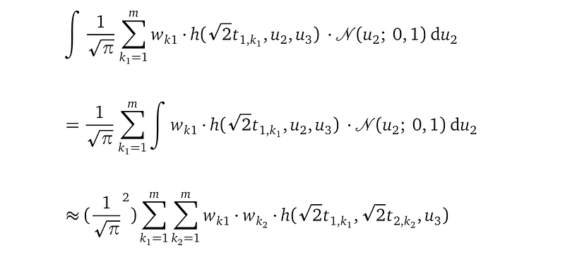
The above expression has m² terms due to the double summation.

We need to apply the Gaussian quadrature rule three times to integrate out all three random variables. After that, we got the final analytical expression for the whole marginal likelihood term:

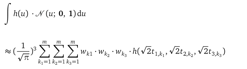
This final approximation has m³ terms.

To generalize this to a data set with n training points, we will have mⁿ number of quadrature terms in the analytical expression that approximates the marginal likelihood term. So the number of terms scales exponentially with the number of data points. It quickly becomes unpractically large. This is why we cannot use Gaussian quadrature to approximate the marginal likelihood term in the Bayes rule.