How to Use Lagrangian Mechanics to Solve Dynamics Problems

An elegantly simple step-by-step process to solve conservative dynamics problems (shown w/ example)

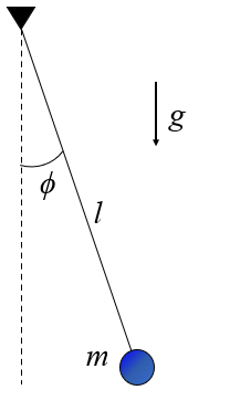
If you are like most engineering or physics students, you’ve had at least one course that involved those troublesome dynamics problems. Maybe you are in that class right now, seeking help from the internet. Most students find these exercises to be challenging, so you are not alone. Hopefully this article will help in your pursuit of solving dynamic systems. At the end of this article, you’ll have a sound procedure to use Lagrangian mechanics to arrive at your system’s equations of motion. In order to demonstrate this process, we will use a simple pendulum problem (see image above).

1. Knowns and Unknowns

To begin solving a dynamic system, we need a solid foundation to begin with. We should determine what we know and what we don’t before rushing into our problem. Our known values are typically stated in a problem statement (if using a textbook) or are values that can be measured (if it is a real-life problem). For our simple pendulum problem, we will consider a known mass, m, at the end of a massless, rigid rod of known length, L. Additionally, for some problems, we also might have to make reasonable assumptions. In our problem, we will consider gravity, g, to be constant and the pivot point to be frictionless (not the best assumption, but it will do).

Now that our knowns are laid out, we need our unknowns, or what we are looking for in a particular problem. For our simple pendulum problem, this would be how the mass of the pendulum moves. We are looking for a way to describe the motion of the mass. This could be defined any number of ways, but the easiest would be how the angle, ϕ, evolves over time, or ϕ(t). Because our system has one degree of freedom (since we have a rigid rod), the angle fully defines where the mass is located.

2. Adding Coordinate System(s)

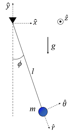
The next step is to set up a coordinate system or systems that best fit our problem. Since our pendulum has a swinging motion, a rotating coordinate system (r-θ axes) that moves with the mass would suit our system best. We also should define an inertial frame (x-y axes) at the pivot point to later define our potential energy. By the right-hand rule for both coordinate systems, we can also define z axis out of the page. Here is what our coordinate systems would look like:

3. Defining the Lagrangian for the System

With our coordinate system defined, we can begin to create the Lagrangian to later be used to obtain our equations of motion. The Lagrangian is defined as follows:

In this equation, L is the Lagrangian (not to be confused with the pendulum length, l). The Lagrangian is defined as the difference of the kinetic energy, T, and the potential energy, V, of the system of interest. For us, the system is the mass, m. In other problems, there could be multiple masses involved.

For the kinetic energy, we use the tangential velocity of the mass (since it has only a rotational motion). We can also obtain the velocity for the mass using kinematics, specifically the basic kinematic equation, as follows:

Note the superscript I represents our inertial frame and R represents our rotating frame. When used with a time derivative, our superscripts mean we need to take our derivative in that frame of reference. This equation results in the tangential velocity for our mass, as expected. Since we do not have a spring or another conservative force, we only need to consider gravitational potential energy. We can use ϕ and l to define our height, h, from the pivot point (note that it is negative since we are below the pivot).

Subtracting those two, the Lagrangian becomes:

4. Using the Euler-Lagrange Equation to Derive the Equations of Motion

By using ϕ to define our mass’ location (and not a set of Cartesian coordinates, x and y), we simplify our math substantially. Once you obtain the Lagrangian, the next step is to use the Euler-Lagrange equation of the following form:

Note that this equation is only valid for a conservative system. Meaning, we can only use it for systems that do not have a dissipative force (e.g. friction). We can solve these derivatives pretty simply as shown below using the Lagrangian we defined in Step 3:

Note: if you have more than one coordinate, you should use the Euler-Lagrange equation on each coordinate, q. The generalized form of the equation is:

Back to our problem, we can combine the derivatives and perform some algebra to arrive at our equation of motion for the mass in terms of the angle, ϕ, and problem constants:

This equation can be solved using a numerical solver, or if a small angle approximation (sinϕ ~= ϕ) is made, an analytical expression can be derived to describe how the angle, ϕ, changes in time. Either way you decide to solve it, you now have the framework to solve conservative dynamics problems using Lagrangian mechanics.

That’s all for this explanation. If you have any questions, feel free to comment. I’d be more than happy to help. Thank you!

If you want to learn to numerically integrate equations of motion, check out my other article: