Using Keras Reinforcement Learning API with OPENAI GYM

This tutorial focuses on using the Keras Reinforcement Learning API for building reinforcement learning models. To get an understanding of what reinforcement learning is please refer to these articles on DataCamp.

In this tutorial, you will learn how to use Keras Reinforcement Learning API to successfully play the OPENAI gym game CartPole..

To Learn more about the GYM toolkit, visit

By the end of this tutorial, you will know how to use 1) Gym Environment 2) Keras Reinforcement Learning API

Assuming that you have the packages Keras, Numpy already installed, Let us get to installing the GYM and Keras RL package. Do this with pip as

pip install gym

pip install keras-rl

Import the following into your workspace

import gym
import random
import numpy as np
from keras.layers import Dense, Flatten
from keras.models import Sequential
from keras.optimizers import Adam

Specifying the environment name to the make method of gym will load the environment to your workspace. Load the Cart Pole environment from gym with

env = gym.make('CartPole-v1')

To get an idea about the number of variables affecting the environment, do

states = env.observation_space.shape[0]
print('States', states)

For the cart pole environment the input variables are position, velocity, angular position and angular velocity. To get an idea about the number of possible actions in the environment, do

actions = env.action_space.n
print('Actions', actions)

For the cart pole environment the responses are left and right.

There are three methods of the environment you should be familiar with

1) step() — This helps you execute an action by returning the (next_state, reward, done, info) resulting from that action. Where next_state — Indicates new state of the environment as a result of the step reward — Indicates the reward for that step done — indicates if you lost the game info — Gives system related info 2) render() — When called visualizes each step

3) reset() — Helps you reset the game returning a new state.

Let us now play 10 games / episodes and during each game we take random actions between left and right and see what rewards we get.

episodes = 10

for episode in range(1,episodes+1):
    # At each begining reset the game 
    state = env.reset()
    # set done to False
    done = False
    # set score to 0
    score = 0
    # while the game is not finished
    while not done:
        # visualize each step
        env.render()
        # choose a random action
        action = random.choice([0,1])
        # execute the action
        n_state, reward, done, info = env.step(action)
        # keep track of rewards
        score+=reward
    print('episode {} score {}'.format(episode, score))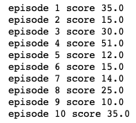

We see that we lost the game very quickly in each of the 10 games.

We will use the SARSA Agent and Epsilon Greedy Q policy to train our reinforcement learning model. To know more about the policies and the agents, please refer to other DataCamp reinforcement learning tutorials mentioned in the beginning of this tutorial.

Let us now define a simple keras model which will have 4 input neurons to accept the 4 state information and 2 output neurons with linear activation which will return the maximum possible reward to the two possible actions. Between the input and the output layers we have 3 Dense layers with 24 neurons and activation as relu.

def agent(states, actions):
    model = Sequential()
    model.add(Flatten(input_shape = (1, states)))
    model.add(Dense(24, activation='relu'))
    model.add(Dense(24, activation='relu'))
    model.add(Dense(24, activation='relu'))
    model.add(Dense(actions, activation='linear'))
    return model
  
model = agent(env.observation_space.shape[0], env.action_space.n)

Import the Agent and the policy as

from rl.agents import SARSAAgent
from rl.policy import EpsGreedyQPolicy

policy = EpsGreedyQPolicy()

We define the SARSA agent by specifying the model, policy and the nb_actions paramaters. Where the model is the keras model we have defined, the policy is EpsGreedyQPolicy and nb_actions is 2.

sarsa = SARSAAgent(model = model, policy = policy, nb_actions = env.action_space.n)

Compile the sarsa agent with mean squared error loss and adam optimizer.

sarsa.compile('adam', metrics = ['mse'])

We then fit it by specifying the environment and the number of steps you want to train it for.

sarsa.fit(env, nb_steps = 50000, visualize = False, verbose = 1)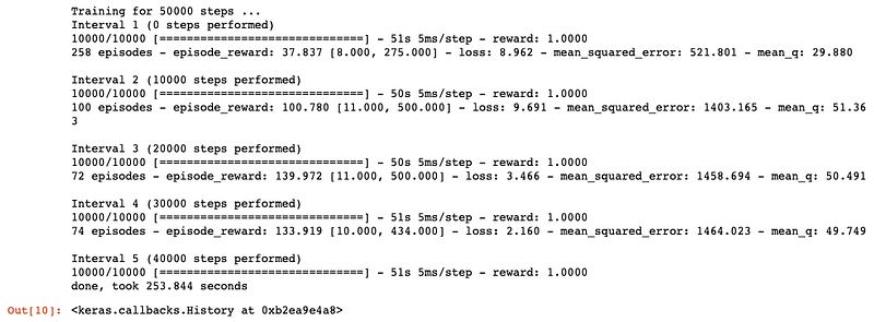

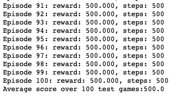
With the training done, we will test it for 100 episodes and see what scores we get.

scores = sarsa.test(env, nb_episodes = 100, visualize= False)
print('Average score over 100 test games:{}'.format(np.mean(scores.history['episode_reward'])))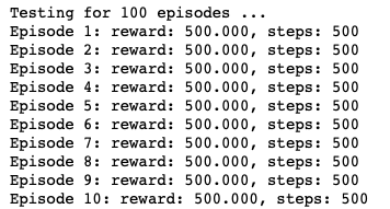

Save trained agent weights with…

sarsa.save_weights('sarsa_weights.h5f', overwrite=True)

If needed, one can load the saved weights with…

# sarsa.load_weights('sarsa_weights.h5f')

To finish off the tutorial, let us visualize the game as played by the trained agent. Setting visualize parameter to true is important to visualize the game.

_ = sarsa.test(env, nb_episodes = 2, visualize= True)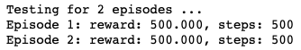

The code and the wights file for this tutorial can be found at

https://github.com/anagar20/Keras-Reinforcement-Learning-API-Cart-Pole-