Using Google Earth Engine (GEE), utilise the Sentinel-2 imagery to generate the Enhanced Vegetation Index (EVI)

EVI from Sentinel-2 image on GEE

What is Enhanced Vegetation Index (EVI)?

The Enhanced Vegetation Index (EVI) is a vegetation index that improves upon the Normalized Difference Vegetation Index (NDVI) by decoupling the canopy background signal and minimizing atmospheric interference. It offers greater sensitivity in regions with high biomass and enhances vegetation monitoring capabilities.

The EVI, obtained from Landsat or Sentinel-2 images, provides a measure of vegetation greenness similar to the NDVI. However, the EVI takes into account distortions caused by airborne particles and ground cover beneath the vegetation, which can affect the reflected light. This adjustment allows the EVI to provide more accurate data in areas with dense vegetation, such as rainforests, without saturating as quickly as the NDVI.

EVI Versus NDVI

In comparison to NDVI, EVI offers several advantages:

1. Sensitivity to high biomass areas: EVI exhibits higher sensitivity to changes in regions with high biomass, addressing a significant limitation of NDVI. This means that EVI can more accurately capture variations in vegetation in densely vegetated areas.
2. Reduced atmospheric impact: EVI takes measures to minimize the influence of atmospheric conditions on vegetation index values. By accounting for atmospheric interference, EVI provides a clearer representation of the actual vegetation signal.
3. Adjustment for canopy background signals/noise: EVI incorporates adjustments to account for canopy background signals or noise, further refining the accuracy of the vegetation index. This adjustment helps separate the vegetation signal from other factors that can affect the index values.
4. Sensitivity to canopy characteristics: EVI demonstrates greater sensitivity to changes in plant canopy attributes, such as leaf area index (LAI), canopy structure, plant phenology, and stress. In contrast, NDVI primarily responds to the amount of chlorophyll present in vegetation.

Enhanced Vegetation Index (EVI) Formula

The Enhanced Vegetation Index (EVI) incorporates additional components to enhance its calculation. It includes an “L” value for canopy background, “C” values for air resistance coefficients, and blue band (B) values. By incorporating these improvements, the EVI calculates the index as a ratio of the red (R) and near-infrared (NIR) values while minimizing the impact of background noise, ambient noise, and saturation. These enhancements contribute to a more accurate and reliable measurement of vegetation dynamics.

EVI = G * ((NIR - R) / (NIR + C1 * R – C2 * B + L))

The output range of EVI calculation typically varies from 0.0 to 1.0.

Calculation of EVI for Sentinel 2 in Google Earth Engine (GEE)

Here’s a step-by-step Python code snippet for computing the Enhanced Vegetation Index (EVI) using Google Earth Engine (GEE) in a Jupyter notebook:

Import Libs:

# Import libs
import geemap, ee
import geemap.colormaps as cm
# initialize our map
Map = geemap.Map()

Set Area Of Interest for calculation:

# get our Ho Chi Minh, Vietnam
# I have taken level 1 data for country data from FAO datasets
aoi = ee.FeatureCollection("FAO/GAUL/2015/level1") \
   .filter(ee.Filter.eq('ADM1_NAME',"Ho Chi Minh City")).geometry() 

Define function for EVI calculations:

def getEVI(image):
    # Compute the EVI using an expression.
    EVI = image.expression(
        '2.5 * ((NIR - RED) / (NIR + 6 * RED - 7.5 * BLUE + 1))', {
            'NIR': image.select('B8').divide(10000),
            'RED': image.select('B4').divide(10000),
            'BLUE': image.select('B2').divide(10000)
        }).rename("EVI")

    image = image.addBands(EVI)

    return(image)

Date of image, addition in image collection as a properties

def addDate(image):
    img_date = ee.Date(image.date())
    img_date = ee.Number.parse(img_date.format('YYYYMMdd'))
    return image.addBands(ee.Image(img_date).rename('date').toInt())

Filter the image and apply the EVI computation formula

# filter sentinel 2 images and apply the EVI formula, finally we obtain 
# single image with median operation

Sentinel_data = ee.ImageCollection('COPERNICUS/S2_SR') \
    .filterDate("2023-03-01","2023-03-31").filterBounds(aoi) \
    .map(getEVI).map(addDate).median()

Add layers to map and visualise it.

# set some thresholds
#  A nice EVI palette
palett = [
    'FFFFFF', 'CE7E45', 'DF923D', 'F1B555', 'FCD163', '99B718',
    '74A901', '66A000', '529400', '3E8601', '207401', '056201',
    '004C00', '023B01', '012E01', '011D01', '011301']

pall = {"min":0.1, "max":0.8, 'palette':palett}



Map.centerObject(aoi)
Map.addLayer(Sentinel_data.clip(aoi).select('EVI'), pall, "EVI")

Map.addLayerControl()
Map

The figure below illustrates the expected output:

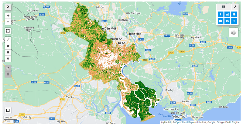
Get all the code in GitHub in the format of Jupyter Notebook.

Stay Connected

If you enjoyed this article, we invite you to become a Medium member and gain access to thousands of similar articles.

Thanks for reading.