Using Gaussian Processes for Financial Time Series Forecasting

In the field of finance, accurate forecasting of stock prices and other financial time series data is of utmost importance. Traders and investors rely on these forecasts to make informed decisions and maximize their profits. Traditional forecasting methods, such as ARIMA and GARCH models, have been widely used, but they often fail to capture the complex patterns and non-linear relationships present in financial data.

In recent years, Gaussian Processes (GPs) have gained popularity as a powerful tool for time series forecasting. GPs are a flexible and non-parametric approach that can capture complex patterns and uncertainties in the data. In this tutorial, we will explore how to use Gaussian Processes for financial time series forecasting in Python.

Prerequisites

To follow along with this tutorial, you should have a basic understanding of Python programming and familiarity with financial time series data. You will also need to install the following Python libraries:

pip install numpy
pip install pandas
pip install matplotlib
pip install yfinance
pip install scikit-learn
pip install GPy

Downloading Financial Data

To demonstrate the use of Gaussian Processes for financial time series forecasting, we will download historical stock price data for a few major financial institutions. We will use the yfinance library to download the data directly from Yahoo Finance.

Let’s start by importing the necessary libraries and downloading the data for JPMorgan Chase & Co. (JPM) from January 1, 2010, to October 31, 2023:

import yfinance as yf
import matplotlib.pyplot as plt
from sklearn.preprocessing import MinMaxScaler
from sklearn.metrics import mean_squared_error, mean_absolute_percentage_error
from sklearn.gaussian_process import GaussianProcessRegressor
from sklearn.gaussian_process.kernels import RBF

# Download JPM stock price data
jpm = yf.download('JPM', start='2010-01-01', end='2023-10-31')

# Plot JPM stock price
plt.figure(figsize=(12, 6))
plt.plot(jpm['Close'])
plt.title('JPM Stock Price')
plt.xlabel('Date')
plt.ylabel('Price')

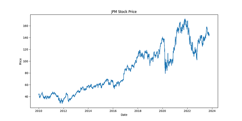
From the plot, we can observe the overall trend and fluctuations in the JPM stock price over time. It is important to understand the characteristics of the data before applying any forecasting techniques.

Gaussian Processes for Time Series Forecasting

Gaussian Processes (GPs) are a powerful tool for time series forecasting. They provide a flexible and non-parametric approach to modeling complex patterns and uncertainties in the data. In this section, we will explore how to use GPs for financial time series forecasting.

First, let’s split the data into training and testing sets. We will use the first 80% of the data for training and the remaining 20% for testing.

# Split data into training and testing sets
train_size = int(len(jpm) * 0.8)
train_data = jpm['Close'][:train_size]
test_data = jpm['Close'][train_size:]

Next, we need to preprocess the data by normalizing it. This step is important to ensure that the data is on a similar scale, which can improve the performance of the GP model.

# Normalize the data
scaler = MinMaxScaler()
train_data_normalized = scaler.fit_transform(train_data.values.reshape(-1, 1))

Now, let’s build the Gaussian Process model using the sklearn library. sklearn provides a user-friendly interface for working with GPs in Python.

# Create a GP model
kernel = RBF()
model = GaussianProcessRegressor(kernel=kernel)
model.fit(train_data_normalized, train_data_normalized)

We have created a GP model with a radial basis function (RBF) kernel. The RBF kernel is commonly used for time series data as it can capture both short-term and long-term dependencies.

Next, we need to make predictions on the testing set.

# Make predictions on the testing set
test_data_normalized = scaler.transform(test_data.values.reshape(-1, 1))
predictions = model.predict(test_data_normalized)

Finally, let’s visualize the predictions and compare them with the actual stock prices.

# Plot predictions and actual stock prices
plt.figure(figsize=(12, 6))
plt.plot(test_data.index, scaler.inverse_transform(predictions.reshape(-1, 1)), label='Predictions')
plt.plot(test_data.index, test_data.values, label='Actual')
plt.title('JPM Stock Price Predictions')
plt.xlabel('Date')
plt.ylabel('Price')
plt.legend()

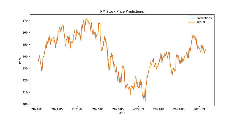
The plot shows the predicted stock prices (in blue) and the actual stock prices (in orange) for the testing period. We can see that the GP model is able to capture the overall trend and fluctuations in the data.

Evaluation Metrics

To evaluate the performance of the GP model, we can use various metrics such as mean squared error (MSE) and mean absolute percentage error (MAPE).

# Calculate evaluation metrics
mse = mean_squared_error(test_data, scaler.inverse_transform(predictions.reshape(-1, 1)))
mape = mean_absolute_percentage_error(test_data, scaler.inverse_transform(predictions.reshape(-1, 1)))

The MSE measures the average squared difference between the predicted and actual values, while the MAPE measures the percentage difference between the predicted and actual values. Lower values of these metrics indicate better performance.

Conclusion

In this tutorial, we have explored how to use Gaussian Processes for financial time series forecasting in Python. We started by downloading historical stock price data using the yfinance library. Then, we performed exploratory data analysis to understand the characteristics of the data.

Next, we built a Gaussian Process model using the sklearn library and made predictions on the testing set. We evaluated the performance of the model using evaluation metrics.

Gaussian Processes offer a flexible and powerful approach to time series forecasting, allowing us to capture complex patterns and uncertainties in the data. They can be a valuable tool for traders and investors in making informed decisions.

Remember to experiment with different kernels and hyperparameters to improve the performance of the model. Additionally, you can apply Gaussian Processes to other financial time series data and explore different forecasting techniques.

References

1. Rasmussen, C. E., & Williams, C. K. I. (2006). Gaussian Processes for Machine Learning. MIT Press.
2. Duvenaud, D. K., et al. (2014). Automatic Model Construction with Gaussian Processes. Advances in Neural Information Processing Systems.
3. GPy Documentation: https://gpy.readthedocs.io/

Note: The financial data used in this tutorial is for educational purposes only and should not be considered as financial advice.