Use This 10-Step Approach to ACE Any Data Analysis

Adding structure to your data analysis

Data analysis is the key to unlocking insights from vast amounts of data. But with more data being generated every day, it’s becoming increasingly challenging to manage and analyze it effectively.

What if I tell you that there was a simpler and more efficient way to analyze your data?

An approach only helps to minimize errors and inconsistencies but also ensures that you achieve your goals with greater accuracy and efficiency. In this blog, we’ll explore a 10-step approach to ace any data analysis project. Whether you’re a seasoned data analyst or just starting out, this approach will provide you with a roadmap to success. So, get ready to take your data analysis skills to the next level!

If you are new to Data Science and want to learn python for data analysis then you can check out my course and get certified: https://bit.ly/3148Qq6

IMDB Dataset

For the illustration purpose, we will pick the IMDB dataset for the top 1000 movies to understand the features/traits of top IMDB movies by applying the 10 steps process. The dataset has been take from kaggle, you can download it here.

Let’s start with the process:

STEP 1: Summary

The first step is to get the summary of columns present in the dataset, but before that, we will import the packages and read our IMDB dataset.

The summary helps us to understand the data by showing the statistics (count, number of unique values, top, mean, etc) for the columns as shown below:

# import our packages 
import pandas as pd 
import matplotlib.pyplot as plt

# reading the data
df_movies =  pd.read_csv('imdb_top_1000.csv')

# summary of the columns   
df_movies.describe(include = 'all')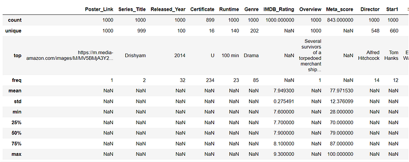

Some takeaways:

• Drishyam occurs twice in the top 1000 IMDB movies (One of the movies is in Malayalam and another is in Hindi).
• Most of the movies(32) are from 2014.
• The drama genre has most(85) movies.
• Alfred Hitchcock has most(14) movies in the top 1000.
• We can also see the distribution(min,25%,50%…etc) of IMDB ratings across these movies.

STEP 2: Data Types

Step 2 is to do a sanity checks of the data types of the columns of the dataframe. If we find some incorrect data types then we will correct them in this step.

print(df_movies.dtypes)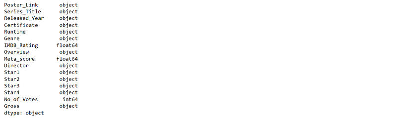

We can see that Released_Year, Runtime, Gross are object data types and should have been int64. Let’s convert the data types into int64:

# convert release year into int
df_movies.loc[df_movies.Released_Year == 'PG','Released_Year'] = '9999'
df_movies['Released_Year'] = df_movies['Released_Year'].astype(int)

# Gross into int
df_movies['Gross'] = df_movies['Gross'].str.replace(',','')
df_movies['Gross'] = df_movies['Gross'].fillna(0).astype(int)

# runtime into int 
df_movies['Runtime'] = df_movies['Runtime'].str.replace(' min','').astype(int)
df_movies.dtypes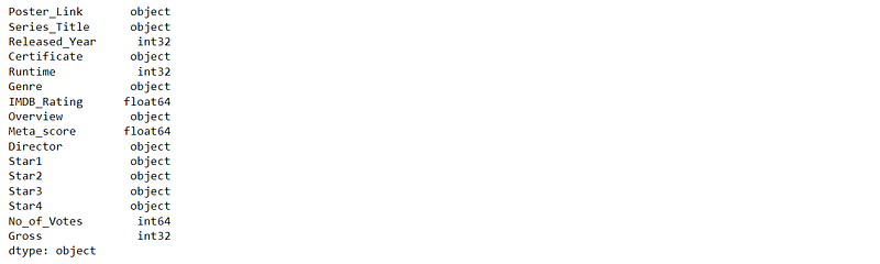

STEP 3: Missing values

The 3rd step is to find the number of missing values across the columns of the dataframe. It’s important to understand the count of nulls so that we can gauge whether we need to treat them.

# find nulls 
df_movies.isnull().sum()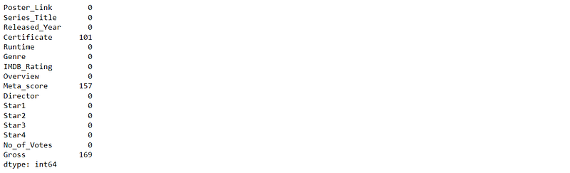

If majority of the values(>70%) within a column are nulls, we can drop the column, else if only a few values are nulls(<20%), we can do missing value treatment.

STEP 4: Missing values treatment

Once we know the count of missing values, the next step is to treat the columns with missing values.

For illustration purposes, I am filling the nulls with the mean value of the columns, although there are more sophisticated methods of missing value treatment.

# let's replace the nulls with mean 
df_movies['Meta_score'].fillna(df_movies['Meta_score'].mean())
df_movies['Gross'].fillna(df_movies['Gross'].mean())
df_movies.head()

STEP 5: Outliers

The step 5 is to check for outliers. There are multiple ways of checking the outliers, we will be using the graphical method in this example.

We will pick one continuous variable (meta score) and check for the outlier by looking at the histogram.

# distribution of meta scores 
plt.hist(df_movies['Meta_score'],bins = 15)
plt.show()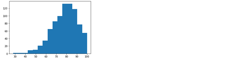

In this example we don’t see any outliers in the meta score as it ranges from 0–100.

STEP 6: Outlier Treatment

Step 6 is to treat the outlier detected in step 5. There are different ways of treating the outliers such as 1) Capping the min and max value limits 2) Removing the rows with outlier values.

Although there is nothing off with the distribution of meta scores, for illustration purposes, let’s cap the minimum meta score value to 40.

# capping the minimum meta score to 40
df_movies.loc[df_movies['Meta_score'] < 40,'Meta_score'] = 40

#check the minimum score 
df_movies['Meta_score'].min()
# output : 40.0

STEP 7: Who — A person, member etc.

Step 7 is to answer the questions related to a person, member, etc. For example in our use case, we have actors and directors and we can formulate and answer the following question related to them.

• Who has directed the most number of top IMDB movies? (univariate)
• Who has acted in most top IMDB movies? (univariate)
• Which Actor-Director combination gave most top IMDB movies? (bivariate)
• Who gave music in most top IMDB movies ? (Data not available)
• And More …..

Now, let’s answer these questions.

## Who has directed the most number of top IMDB movies ?
df_movies.groupby(['Director']).agg({'Series_Title':'count'}).reset_index().rename(columns = {'Series_Title':'count'}).\
sort_values('count',ascending = False).head(5)

## Who has acted in the most number of top movies 
df_movies.groupby(['Star1']).agg({'Series_Title':'count'}).reset_index().rename(columns = {'Series_Title':'count'}).\
sort_values('count',ascending = False).head(5)

## Director - Actor works best 
df_movies.groupby(['Director','Star1'])['Series_Title'].count().reset_index().\
rename(columns = {'Series_Title':'Count'}).sort_values('Count',ascending = False).head(5)

STEP 8: When — time related questions!

Step 8 is to answer questions related to the time aspect- year, month, week, etc. In the context of our data, we can find the following :

• Find the years with most movies in IMDB top 1000 ? (univariate)

# finding years with most movies in top 1000
year_dis = df_movies.groupby('Released_Year')['Series_Title'].count().reset_index().\
rename(columns = {'Series_Title':'Count'}).sort_values('Count',ascending = False).head(10)

plt.bar(year_dis['Released_Year'].astype(str), year_dis['Count'], width = 0.5)
plt.xlabel('Years')
plt.ylabel('Number of Movies')
plt.title('Years with most movies in IMDB top 1000')
plt.show()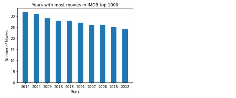

STEP 9: Where — Place related questions!

Step 9 is to look at the things from the “place” perspective, for example, country, state, regions etc. In context to our data set, we can find the following :

• Find countries with most movies in IMDB top 1000.

Currently, we don’t have the data to answer this question.

While formulating these questions, I would recommend you to be as exhaustive as possible and don’t limit the thought process based on data availability because the data that is not available now could be obtained later.

STEP 10: What/Which

Step 10 is about formulating questions about things that are not covered above. These are not related to people, place, time but everything apart from these. This is a bit subjective and takes some time to get used to.

• Which genres are featured most in the top 1000?
• What is the duration of the top movies?
• What is the correlation between the rating and gross earning?
• and more…

For illustration purposes, we are answering the first question using the following code:

### Which genres are featured most in top 1000 ? 
genre_dis = df_movies.groupby('Genre')['Series_Title'].count().reset_index().\
rename(columns = {'Series_Title':'Count'}).sort_values('Count',ascending = False).head(5)
fig, ax = plt.subplots()
plt.bar(genre_dis['Genre'], genre_dis['Count'], width = 0.5)
plt.setp(ax.get_xticklabels(), rotation=30, horizontalalignment='right')
plt.show()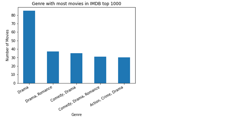

I hope you get an idea of how to implement the 10-step process to perform the data analysis.

Conclusion

In conclusion, a structured approach to data analysis is essential for anyone looking to make informed decisions based on data. By following the 10-step approach outlined in this blog, you’ll be well equipped to tackle even the most complex data analysis projects with confidence. Whether you’re a seasoned data analyst or just starting out, this approach will help you to avoid common pitfalls and maximize your productivity.

Thank You!

If you find my blogs useful, then you can follow me to get direct notifications whenever I publish a story.

If you like to access all the amazing stories on Medium, consider supporting me and thousands of other writers by signing up for a membership. It only costs $5 per month, it supports us, writers, greatly.