
Use machine learning to predict on the price of gems

I was a bit surprised yesterday when I happened to look on the competitions page of the Kaggle website to find that two playground competitions were running concurrently. I therefore scrambled to enter the competition and write the code for it. This particular competition was a regression problem concerning gemstones, and the problem statement for it is written below:-
I wrote the code on the Python programming language and used Kaggle’s free Jupyter Notebook to do so.
Once the program was created, I imported the libraries I would need to execute the program, being:-
- Numpy to perform numerical computations,
- Pandas to perform data processing,
- Os to go into the operating system,
- Xgboost to train, fit the data into the model,
- Sklearn to perform machine learning operations,
- Matplotlib to visualise the data, and
- Seaborn to statistically visualise the data.
The os library in Python is a built-in module that provides a way to interact with the underlying operating system in a portable way. The primary purpose of the os library is to provide a platform-independent way to perform operating system related tasks, such as file and directory operations, process management, environment variables, and system information.
Some common tasks that can be performed with the os library in Python include:
- Creating, renaming, and deleting files and directories
- Retrieving information about a file or directory, such as its size, creation time, and modification time
- Changing the current working directory and navigating the file system
- Executing external commands and programs
- Managing processes and subprocesses
- Setting and retrieving environment variables
- Retrieving system information, such as the name of the current user, the host name, and the current operating system
Overall, the os library is a powerful tool that allows Python programmers to interact with the underlying operating system and perform a wide range of system-level tasks.
Once the libraries were loaded, I used os to go into the directory and retrieve the files that would be used in it:-
I then used pandas, which is a library used for data processing, to read the three csv files retrieved by the os library, and converted them to dataframes, being train, test and submission:-
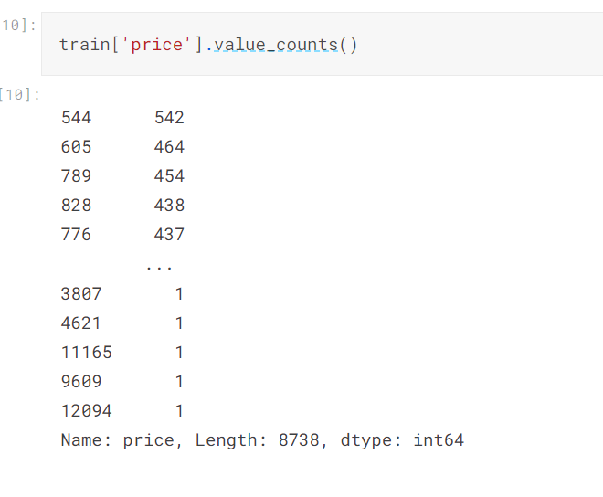
I analysed the target by performing a count of all of the values in it:-
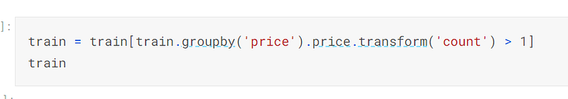
I removed all of the rows that had only one occurrence because they would add no meaning to the training process:-
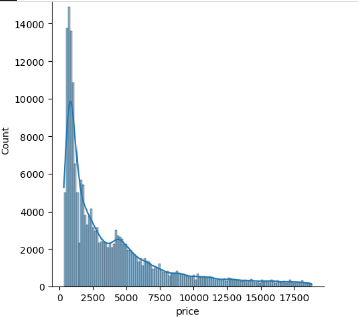
I visualised the target and ascertained that it is skewed:-
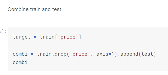
I defined the target as being the price.
I then created one dataframe by dropping the price from train and appending test to it:-
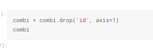
I then dropped the ‘id’ column from combi because each row in the dataframe is indexed already:-
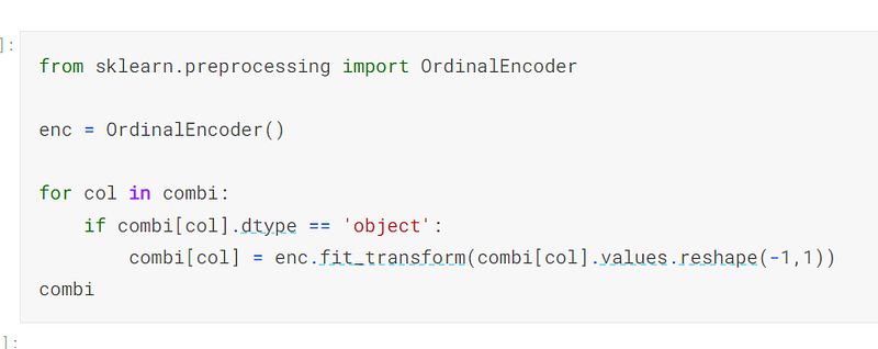
Because three of the columns were of type object, I encoded them using sklearn’s ordinal encoder. (It is important to note that the column of data must be reshaped before it will work.)
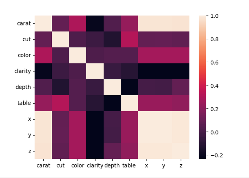
I created a heatmap of the dataframe and noted that three of the columns are highly correlated:-
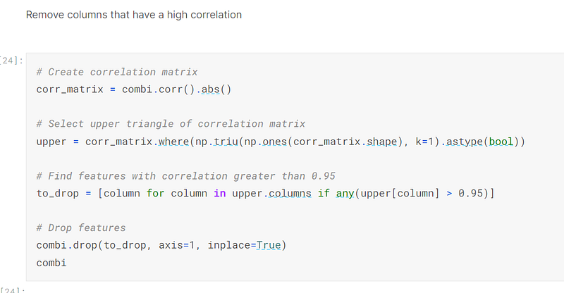
I then removed the three columns that were highly correlated:-
Once the data had been preprocessed, I normalised it by converting the cells to values between 0 and 1.
Normalisation in machine learning refers to the process of rescaling numerical features to a common scale, without distorting differences in the ranges of values or losing information. Normalisation is an important preprocessing step in machine learning, as it can improve the performance and accuracy of many machine learning models.
The reason why normalisation is necessary is that different features in a dataset may have different scales, which can cause some algorithms to give undue importance to certain features. For example, if one feature has a range of values from 0 to 100 and another feature has a range of values from 0 to 1, then the algorithm may give more importance to the first feature, simply because its values are larger in magnitude. Normalisation helps to prevent this issue and ensures that all features contribute equally to the learning process:-
I then defined the independent and dependent variables, as being X and y respectively.
In machine learning, the dependent variable, also known as the target variable, is the variable that is being predicted or modelled. The independent variables, also known as the predictor variables, are the variables that are used to make the prediction or model the outcome.
In a machine learning algorithm, the goal is to find a relationship between the independent variables and the dependent variable that can be used to make accurate predictions on new data. This is typically done by training a model on a dataset that includes both the independent variables and the known values of the dependent variable. Once the model has been trained, it can be used to make predictions on new data where the value of the dependent variable is unknown.
I then attached the target to the X variable and split the dataset into training and validating sets.
Splitting a dataset into training and validation sets is a crucial step in machine learning because it allows us to evaluate the performance of our model on data that it has not seen before.
When building a machine learning model, the goal is to create a model that can generalise well to new, unseen data. In other words, we want the model to be able to make accurate predictions on data that it has not been trained on. If we were to evaluate the model on the same data that we used to train it, we would not be able to accurately assess how well the model would perform on new data.
To address this issue, we split the dataset into two parts: a training set and a validation set. The training set is used to train the model, while the validation set is used to evaluate the performance of the model on data that it has not seen before.
By splitting the dataset in this way, we can tune the hyperparameters of the model (e.g., the learning rate or regularisation strength) on the validation set and ensure that the model is not overfitting to the training set. Overfitting occurs when the model performs well on the training set but does not generalise well to new data.
Overall, splitting the dataset into training and validation sets is a critical step in machine learning that allows us to build models that can generalise well to new data and avoid overfitting.
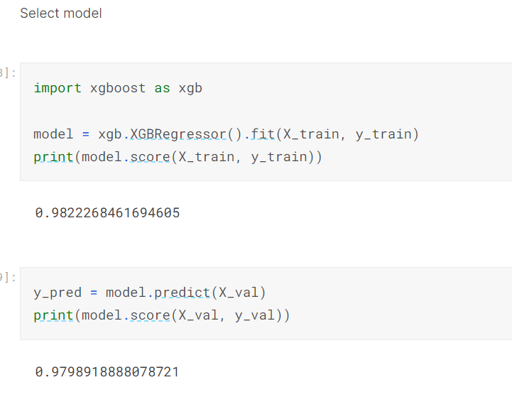
Once the data had been preprocessed, normalised, and split, I selected the model I would use, in this instance being XGBRegressor.
XGBoost (Extreme Gradient Boosting) is a popular gradient boosting framework used for building high-performance machine learning models. XGBRegressor is a specific implementation of XGBoost that is used for regression problems.
XGBRegressor works by combining multiple weak regression models into a single, strong model. It does this by iteratively adding decision trees to the model and updating the weights of the training samples to focus on the samples that were previously misclassified. The process of adding decision trees and updating weights is repeated until the model’s performance reaches a desired level or until a specified number of trees have been added.
During the training process, XGBRegressor uses gradient boosting to optimise the objective function, which is a measure of the difference between the predicted and actual values of the dependent variable. The gradient boosting algorithm minimises this objective function by adjusting the weights of the training samples and the parameters of the decision trees.
Some of the key hyperparameters of XGBRegressor include the learning rate (the step size taken during each iteration of gradient boosting), the maximum depth of the decision trees, and the regularisation parameters used to prevent overfitting.
Once the XGBRegressor model has been trained, it can be used to make predictions on new data. The model takes in the independent variables as input and outputs a predicted value for the dependent variable. The performance of the model can be evaluated using various metrics, such as the mean squared error or R-squared.
Overall, XGBRegressor is a powerful tool for building high-performance regression models, particularly in situations where the dataset has many features and complex relationships between the independent and dependent variables.
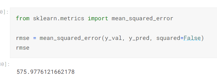
When the data had been trained and fitted into the model, and the validation set had been predicted on, I used sklearn’s mean_squared_error to find the root mean squared error.
Root Mean Squared Error (RMSE) is a commonly used metric to evaluate the accuracy of a machine learning model’s predictions, particularly in regression problems. It measures the difference between the predicted and actual values of the dependent variable and provides a measure of how well the model is able to make predictions.
RMSE is calculated by taking the square root of the average of the squared differences between the predicted and actual values. Mathematically, it can be expressed as:
RMSE = sqrt(1/n * sum(i=1 to n) (y_i — y_pred,i)²)
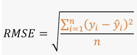
where n is the number of observations in the dataset, y_i is the actual value of the dependent variable for the ith observation, and y_pred,i is the predicted value of the dependent variable for the ith observation.
The square of the differences is used in the calculation to ensure that positive and negative errors do not cancel each other out. Taking the square root of the average of these squared differences provides a measure of the typical or average difference between the predicted and actual values.
A lower RMSE indicates that the model is making more accurate predictions, while a higher RMSE indicates that the model is making less accurate predictions. RMSE is particularly useful when the dataset has outliers, as it is less sensitive to them compared to other metrics like mean absolute error.
Overall, RMSE is a useful metric for evaluating the accuracy of a regression model’s predictions and can be used to compare the performance of different models.
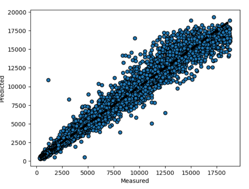
I then plotted the predicted values against the actual values. The plot did not look too bad, but there were a few outliers present:-
I then made predictions on the test set:-
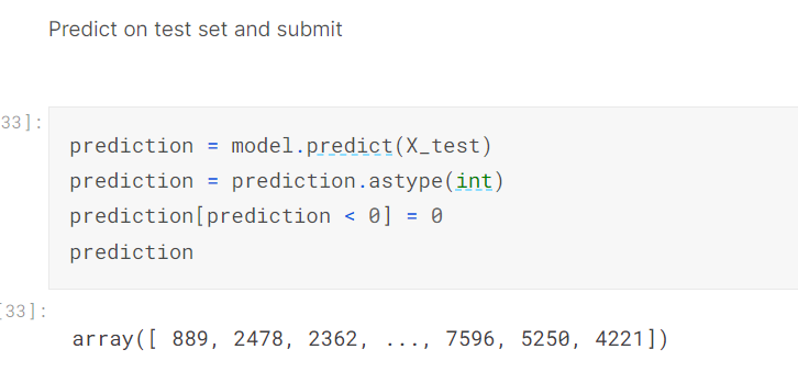
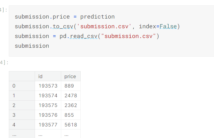
And finally, I prepared the predictions to be submitted to Kaggle for scoring:-
- The prediction was placed in the price column of the submission dataframe.
- Pandas was used to convert the dataframe to a csv file, called submission.csv.
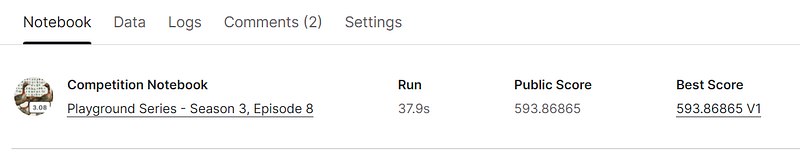
I then submitted the csv file to Kaggle to be scored. At the time of this writing I am 126 out of 190 teams.:-
Of course, there is more that I can do to improve my score, such as trying out a different model. Time permitting, I will soon be looking to using different models, and I will certainly post the results on medium.
I have created a code review to accompany this blog post, which can be viewed here:- https://www.youtube.com/watch?v=vUmUSHqbiqM


