Unveiling U-Net++: A Hands-On Guide on Image Segmentation

Imagine looking at an image and being able to decipher distinct regions, each representing a unique object or area of interest.

Whether you’re a computer vision researcher striving to create innovative medical diagnostic tools, or an engineer developing next-generation autonomous vehicles capable of perceiving their surroundings, image segmentation is an enthralling and intricate field with applications spanning a wide array of industries.

In this blog post, we’ll embark on an exploration of the captivating world of image segmentation and its diverse use cases. We’ll dive deep into the U-Net architecture, a groundbreaking development in image segmentation, before unveiling the secrets of U-Net++, an enhanced version that achieves exceptional results. Regardless of whether you’re a seasoned computer vision expert or just beginning your journey, this hands-on guide to U-Net++ will offer valuable insights!

Introduction to Image Segmentation and Its Use Cases

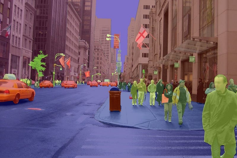
Image segmentation is a cornerstone of computer vision. The objective is to partition images into multiple non-overlapping segments, with each segment representing a distinct object or region of interest. By transforming raw pixel data into meaningful components, image segmentation allows computer vision systems to reason about and process complex scenes more effectively.

The power of image segmentation can be harnessed for an array of use cases across various industries:

1. Medical Imaging: Image segmentation plays a critical role in diagnosing and monitoring diseases by enabling the precise delineation of anatomical structures, abnormalities, and lesions in medical images, such as CT scans, MRIs, and X-rays.
2. Autonomous Vehicles: In the realm of self-driving cars, image segmentation contributes to a better understanding of the vehicle’s surroundings, by distinguishing roads, pedestrians, other vehicles, and traffic signs, facilitating safe and efficient navigation.
3. Robotics: Image segmentation aids robots in tasks such as object recognition, manipulation, and obstacle avoidance by isolating objects of interest and discerning them from the background.
4. Remote Sensing: Satellite and aerial imagery can be segmented to analyze land use, vegetation, and urban planning, providing valuable insights for environmental monitoring, disaster management, and resource management.
5. Video Surveillance: In security applications, image segmentation can track and identify objects or individuals in real-time, thereby enhancing safety and crime prevention.
6. Augmented Reality: Image segmentation enables the seamless integration of virtual objects into real-world scenes, enriching user experiences in gaming, education, and navigation.

With the increasing demand for advanced computer vision systems, image segmentation continues to evolve, giving rise to innovative techniques and architectures, such as the powerful U-Net++ that we will explore in this blog post.

The Original U-Net Architecture — An overview

U-Net is a pioneering architecture in the field of image segmentation, was introduced by Olaf Ronneberger, Philipp Fischer, and Thomas Brox in their 2015 paper, “U-Net: Convolutional Networks for Biomedical Image Segmentation”.

The U-net architecture is synonymous with an encoder-decoder architecture. Essentially, it is a deep-learning framework based on FCNs and it comprises two parts:

1. A contracting path similar to an encoder, to capture context via a compact feature map.
2. A symmetric expanding path similar to a decoder, which allows precise localisation. This step is done to retain boundary information (spatial information) despite down sampling and max-pooling performed in the encoder stage.

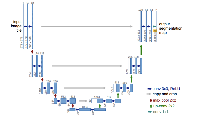
The architecture boasts a unique encoder-decoder structure, reminiscent of an autoencoder, with a fundamental difference: the incorporation of skip connections. These connections bridge the encoder (downsampling) and decoder (upsampling) paths, allowing for seamless fusion of high-level contextual information with low-level spatial details.

This ingenious design enables U-Net to deliver high-quality segmentation results, even when trained on limited amounts of annotated data.

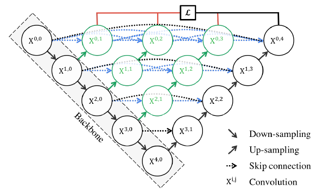
U-Net++: The Evolution of U-Net

U-Net++ is an advanced image segmentation architecture proposed by Zhou et al. in their 2018 paper, “UNet++: A Nested U-Net Architecture for Medical Image Segmentation”. This innovative model builds upon the foundational success of the original U-Net, introducing nested skip connections to create a more robust and powerful segmentation tool.

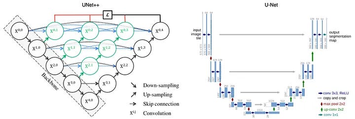
The primary distinction between U-Net and U-Net++ lies in the architecture’s design. While U-Net employs direct skip connections between corresponding encoder and decoder layers, U-Net++ introduces a series of nested skip pathways that bridge the gap between these layers. This nested structure enables the model to iteratively refine and fuse features from multiple resolution levels, enhancing the model’s localization accuracy and feature expressiveness.

The nested skip pathways in U-Net++ help address the following challenges in the original U-Net:

1. Improved feature fusion: U-Net++ facilitates the fusion of high-level contextual information with low-level spatial details more effectively, resulting in more accurate segmentations.
2. Enhanced localization: U-Net++ provides better localization of objects and boundaries by integrating multi-resolution features, which proves particularly beneficial for segmenting objects with varying sizes and shapes.

Performance comparisons between U-Net and U-Net++ demonstrate that the latter exhibits superior segmentation capabilities in various applications.

Deep Supervision

Deep supervision is another crucial aspect of the U-Net++ architecture, contributing significantly to its improved performance in image segmentation tasks. Deep supervision involves the introduction of auxiliary supervision at various levels of the network, enabling the model to learn more effectively by providing intermediate feedback during the training process.

In the context of U-Net++, deep supervision is implemented by attaching auxiliary segmentation heads to the nested skip pathways (The red lines in the image above). These segmentation heads generate intermediate segmentation outputs at multiple resolution levels, which are then combined with the final output during the training phase. By leveraging these intermediate outputs, the model is encouraged to produce accurate segmentations at different levels of detail, improving its overall performance.

The benefits of deep supervision in U-Net++ are:

1. Enhanced Gradient Flow: by providing supervision at multiple levels of the network, deep supervision facilitates a more effective flow of gradients during the backpropagation process. This improved gradient flow helps the model learn better representations, particularly for deep layers, which can otherwise suffer from vanishing gradient issues.
2. Regularization Effect: deep supervision acts as a form of regularization, reducing the risk of overfitting. By forcing the model to generate accurate segmentations at different levels of abstraction, it encourages the network to learn more robust and generalizable features, ultimately leading to improved performance on unseen data.

Implementation & hands-on training

Dataset

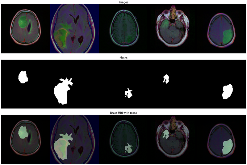
The dataset used in this project is the Brain MRI Segmentation Dataset from Kaggle. The dataset contains 110 images of brain MRI scans with their corresponding segmentation masks. The images are of size 512x512 and the masks are of size 256x256.

The Dataset object can easily be defined as follows:

class BrainDataset(Dataset):
    def __init__(self, df, transform=None):
        self.df = df
        self.transform = transform

    def __len__(self):
        return len(self.df)
    
    def __getitem__(self, idx):

        image = cv2.imread(self.df.iloc[idx, 0])
        image = np.array(image)/255.

        mask = cv2.imread(self.df.iloc[idx, 1], 0)
        mask = np.array(mask)/255.
        
        if self.transform is not None:
            aug = self.transform(image=image, mask=mask)
            image = aug['image']
            mask = aug['mask']
            
        image = image.transpose((2,0,1))
        image = torch.from_numpy(image).type(torch.float32)
        image = T.Normalize((0.485, 0.456, 0.406), (0.229, 0.224, 0.225))(image)
        
        mask = np.expand_dims(mask, axis=-1).transpose((2,0,1))
        mask = torch.from_numpy(mask).type(torch.float32)
        
        return image, mask

Model

Let’s now define the Nested UNet itself.

class conv_block_nested(nn.Module):
    def __init__(self, in_ch, mid_ch, out_ch):
        super().__init__()
        self.activation = nn.ReLU(inplace=True)
        self.conv1 = nn.Conv2d(in_ch, mid_ch, kernel_size=3, padding=1, bias=True)
        self.bn1 = nn.BatchNorm2d(mid_ch)
        self.conv2 = nn.Conv2d(mid_ch, out_ch, kernel_size=3, padding=1, bias=True)
        self.bn2 = nn.BatchNorm2d(out_ch)

    def forward(self, x):
        x = self.conv1(x)
        x = self.bn1(x)
        x = self.activation(x)

        x = self.conv2(x)
        x = self.bn2(x)
        output = self.activation(x)

        return output


class NestedUNet(nn.Module):
    def __init__(self, input_channels=3, num_classes=1, deep_supervision=False):
        super().__init__()

        n1 = 64
        filters = [n1, n1 * 2, n1 * 4, n1 * 8, n1 * 16]
        self.deep_supervision = deep_supervision

        self.pool = nn.MaxPool2d(kernel_size=2, stride=2)
        self.Up = nn.Upsample(scale_factor=2, mode="bilinear", align_corners=True)

        self.conv0_0 = conv_block_nested(input_channels, filters[0], filters[0])
        self.conv1_0 = conv_block_nested(filters[0], filters[1], filters[1])
        self.conv2_0 = conv_block_nested(filters[1], filters[2], filters[2])
        self.conv3_0 = conv_block_nested(filters[2], filters[3], filters[3])
        self.conv4_0 = conv_block_nested(filters[3], filters[4], filters[4])

        self.conv0_1 = conv_block_nested(
            filters[0] + filters[1], filters[0], filters[0]
        )
        self.conv1_1 = conv_block_nested(
            filters[1] + filters[2], filters[1], filters[1]
        )
        self.conv2_1 = conv_block_nested(
            filters[2] + filters[3], filters[2], filters[2]
        )
        self.conv3_1 = conv_block_nested(
            filters[3] + filters[4], filters[3], filters[3]
        )

        self.conv0_2 = conv_block_nested(
            filters[0] * 2 + filters[1], filters[0], filters[0]
        )
        self.conv1_2 = conv_block_nested(
            filters[1] * 2 + filters[2], filters[1], filters[1]
        )
        self.conv2_2 = conv_block_nested(
            filters[2] * 2 + filters[3], filters[2], filters[2]
        )

        self.conv0_3 = conv_block_nested(
            filters[0] * 3 + filters[1], filters[0], filters[0]
        )
        self.conv1_3 = conv_block_nested(
            filters[1] * 3 + filters[2], filters[1], filters[1]
        )

        self.conv0_4 = conv_block_nested(
            filters[0] * 4 + filters[1], filters[0], filters[0]
        )

        if self.deep_supervision:
            self.final1 = nn.Conv2d(filters[0], num_classes, kernel_size=1)
            self.final2 = nn.Conv2d(filters[0], num_classes, kernel_size=1)
            self.final3 = nn.Conv2d(filters[0], num_classes, kernel_size=1)
            self.final4 = nn.Conv2d(filters[0], num_classes, kernel_size=1)
        else:
            self.final = nn.Conv2d(filters[0], num_classes, kernel_size=1)

    def forward(self, x):
        x0_0 = self.conv0_0(x)
        x1_0 = self.conv1_0(self.pool(x0_0))
        x0_1 = self.conv0_1(torch.cat([x0_0, self.Up(x1_0)], 1))

        x2_0 = self.conv2_0(self.pool(x1_0))
        x1_1 = self.conv1_1(torch.cat([x1_0, self.Up(x2_0)], 1))
        x0_2 = self.conv0_2(torch.cat([x0_0, x0_1, self.Up(x1_1)], 1))

        x3_0 = self.conv3_0(self.pool(x2_0))
        x2_1 = self.conv2_1(torch.cat([x2_0, self.Up(x3_0)], 1))
        x1_2 = self.conv1_2(torch.cat([x1_0, x1_1, self.Up(x2_1)], 1))
        x0_3 = self.conv0_3(torch.cat([x0_0, x0_1, x0_2, self.Up(x1_2)], 1))

        x4_0 = self.conv4_0(self.pool(x3_0))
        x3_1 = self.conv3_1(torch.cat([x3_0, self.Up(x4_0)], 1))
        x2_2 = self.conv2_2(torch.cat([x2_0, x2_1, self.Up(x3_1)], 1))
        x1_3 = self.conv1_3(torch.cat([x1_0, x1_1, x1_2, self.Up(x2_2)], 1))
        x0_4 = self.conv0_4(torch.cat([x0_0, x0_1, x0_2, x0_3, self.Up(x1_3)], 1))

        if self.deep_supervision:
            output1 = self.final1(x0_1)
            output2 = self.final2(x0_2)
            output3 = self.final3(x0_3)
            output4 = self.final4(x0_4)
            return [output1, output2, output3, output4]
        else:
            output = self.final(x0_4)
        return output


model = NestedUNet(num_classes=1, deep_supervision=False)

Here’s an overview of the main components in the provided code:

1. conv_block_nested class: This class defines a custom convolutional block used in the Nested U-Net architecture. It consists of two convolutional layers (with kernel size 3 and padding 1), followed by batch normalization layers and ReLU activations. This block takes in the number of input channels (in_ch), intermediate channels (mid_ch), and output channels (out_ch).
2. NestedUNet class: This class defines the Nested U-Net architecture. It takes three optional arguments:

• input_channels: The number of input channels in the input image (default is 3 for RGB images).
• num_classes: The number of output classes (default is 1, for binary segmentation tasks).
• deep_supervision: A boolean flag to enable or disable deep supervision (default is False).

The forward method of the NestedUNet connects all the convolutional blocks with appropriate pooling, upsampling, and concatenation operations. If deep_supervision is enabled, the model outputs predictions at multiple levels of the decoding path. Otherwise, it only outputs the final prediction.

Custom loss function & training loop

I’ve opted for a custom loss function which combines the Dice Loss and a modified Cross-Entropy function.

import torch.nn.functional as F

class CombinedLoss(nn.Module):
    def __init__(self, alpha=0.5):
        super(CombinedLoss, self).__init__()
        self.alpha = alpha

    def forward(self, outputs, targets):
        # Binary Cross Entropy Loss
        bce_loss = F.binary_cross_entropy_with_logits(outputs, targets)

        # Dice Loss
        smooth = 1e-5
        outputs = torch.sigmoid(outputs)
        intersection = torch.sum(outputs * targets)
        union = torch.sum(outputs) + torch.sum(targets)
        dice_loss = 1 - (2 * intersection + smooth) / (union + smooth)

        # Combine the losses
        loss = self.alpha * bce_loss + (1 - self.alpha) * dice_loss
        return loss

You can adjust the alpha parameter to give more weight to either the Binary Cross Entropy loss or the Dice loss.

For the training loop, it’s a boilerplate one:

train_dataset = BrainDataset(train_df, train_transform)
train_dataloader = torch.utils.data.DataLoader(train_dataset, batch_size=32, shuffle=True, num_workers=2)

val_dataset = BrainDataset(val_df, val_transform)
val_dataloader = torch.utils.data.DataLoader(val_dataset, batch_size=32, num_workers=2)

def train_model(train_loader, val_loader, loss_func, optimizer, scheduler, num_epochs):
    loss_history = []
    train_dice_history = []
    train_iou_history = []
    val_dice_history = []
    val_iou_history = []
    
    for epoch in range(num_epochs):
        model.train()
        
        losses = []
        train_dice = []
        train_iou = []
        
        for i, (image, mask) in enumerate(tqdm(train_loader)):
            image = image.to(device)
            mask = mask.to(device)
            outputs = model(image)
            out_cut = np.copy(outputs.data.cpu().numpy())
            out_cut[np.nonzero(out_cut < 0.5)] = 0.0
            out_cut[np.nonzero(out_cut >= 0.5)] = 1.0            
            
            dice = dice_coef_metric(out_cut, mask.data.cpu().numpy())
            iou = iou_metric(out_cut, mask.data.cpu().numpy())
            loss = loss_func(outputs, mask)
            losses.append(loss.item())
            train_dice.append(dice)
            train_iou.append(iou)
            
            optimizer.zero_grad()
            loss.backward()
            optimizer.step()
                
        val_mean_iou = compute_iou(model, device, val_loader)
        val_mean_dice = compute_dice(model, device, val_loader)
        scheduler.step(val_mean_iou)
        loss_history.append(np.array(losses).mean())
        train_dice_history.append(np.array(train_dice).mean())
        train_iou_history.append(np.array(train_iou).mean())
        val_dice_history.append(val_mean_dice)
        val_iou_history.append(val_mean_iou)
        
        print('Epoch : {}/{}'.format(epoch+1, num_epochs))
        print('Training Loss: {:.4f} | Training Dice: {:.4f} | Training IOU: {:.4f} | Validation Dice: {:.4f} | Validation IOU: {:.4f}'.format(loss_history[-1], train_dice_history[-1], train_iou_history[-1], val_dice_history[-1], val_iou_history[-1]))
    return loss_history, train_dice_history, train_iou_history, val_dice_history, val_iou_history


if __name__ == "__main__":

    model = NestedUNet(3, 1, deep_supervision=False).to(device)

    optimizer = torch.optim.Adam(model.parameters(), lr=1e-3)
    scheduler = torch.optim.lr_scheduler.ReduceLROnPlateau(optimizer, 'max', patience=3)
    num_epochs = 20

    combined_loss = CombinedLoss(alpha=0.5)
    history = train_model(train_dataloader, val_dataloader, combined_loss, optimizer, scheduler, num_epochs)
    
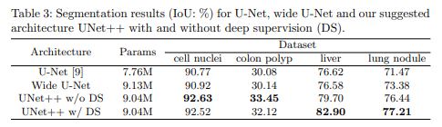
    torch.save(model, 'model.pth')

I’ll leave you to play with different transformations and hyperparameters! Here are the results from the paper:

Conclusion

In conclusion, this article has presented a comprehensive implementation of the UNet++ architecture for medical image segmentation. UNet++ is an enhancement of the original U-Net model, featuring re-designed skip pathways and deep supervision that can potentially improve segmentation performance. We demonstrated the implementation and training of the UNet++ model using a brain MRI dataset for the task of tumor segmentation.

It is important to note that the choice of hyperparameters, loss functions, and optimization methods can greatly impact the performance of the model. Hence, experimenting with different settings and techniques may lead to further improvements in the segmentation results. Additionally, integrating other state-of-the-art techniques, such as attention mechanisms and pre-trained encoders, could potentially enhance the model’s performance even further.

If you liked the post, consider following me on Medium

You can join Artificialis newsletter, here.

You can also support my work directly and get unlimited access by becoming a Medium member through my referral link here!