
Unraveling the 68–95–99.7 Rule in Statistics
Navigating Data with Precision

Introduction
In the vast realm of statistics, where numbers tell stories and trends emerge from data, the 68–95–99.7 Rule stands as a guiding principle. Also known as the empirical rule or the three-sigma rule, this statistical concept provides a quick and powerful way to understand the distribution of data within the framework of the normal distribution curve. Let’s delve into the intricacies of this rule and explore how it shapes the landscape of statistical analysis.
The Essence of the Rule
At its core, the 68–95–99.7 Rule encapsulates the idea that in a normal distribution — a symmetric, bell-shaped curve — a specific percentage of data falls within certain standard deviations from the mean. The rule breaks down these percentages as follows:
Approximately 68% of data falls within one standard deviation.
Around 95% falls within two standard deviations.
An impressive 99.7% is contained within three standard deviations.
Visualizing the Bell Curve
To grasp the significance of the rule, it’s essential to visualize the normal distribution curve. Picture a symmetrical bell-shaped curve where the peak represents the mean (average) of the data. As you move away from the mean in either direction, the percentage of data encompassed by the curve follows the 68–95–99.7 distribution.
# Set seed for reproducibility
set.seed(123)

# Generate a random sample from a normal distribution
data <- rnorm(1000, mean = 0, sd = 1)

# Calculate mean and standard deviation of the data
mean_value <- mean(data)
sd_value <- sd(data)

# Calculate percentages within different standard deviations
within_one_sd <- sum(abs(data - mean_value) < sd_value) / length(data) * 100
within_two_sd <- sum(abs(data - mean_value) < 2 * sd_value) / length(data) * 100
within_three_sd <- sum(abs(data - mean_value) < 3 * sd_value) / length(data) * 100

# Print the results
cat("Percentage within one standard deviation: ", round(within_one_sd, 2), "%\n")
cat("Percentage within two standard deviations: ", round(within_two_sd, 2), "%\n")
cat("Percentage within three standard deviations: ", round(within_three_sd, 2), "%\n")

# Visualize the normal distribution with standard deviation intervals
hist(data, prob = TRUE, col = "lightblue", main = "Normal Distribution with SD Intervals")

# Add lines for mean and standard deviation intervals
abline(v = mean_value, col = "red", lwd = 2)
abline(v = c(mean_value - sd_value, mean_value + sd_value), col = "green", lwd = 2, lty = 2)
abline(v = c(mean_value - 2 * sd_value, mean_value + 2 * sd_value), col = "blue", lwd = 2, lty = 2)
abline(v = c(mean_value - 3 * sd_value, mean_value + 3 * sd_value), col = "orange", lwd = 2, lty = 2)

# Add legend
legend("topright", legend = c("Data", "Mean", "1 SD", "2 SD", "3 SD"), col = c("lightblue", "red", "green", "blue", "orange"), lwd = 2)

# Display the plot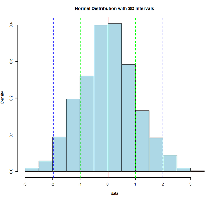
Here, red line is meat at 0, green line is at 1 sigma and b;lue line is at 2 sigma.
Practical Applications
The 68–95–99.7 Rule finds broad applications in various fields. Whether you are analyzing exam scores, manufacturing processes, or economic indicators, understanding the distribution of data within these three standard deviation intervals provides valuable insights. This rule serves as a quick reference for researchers, analysts, and decision-makers.
Quality Control and Process Stability
In quality control and manufacturing, the 68–95–99.7 Rule plays a pivotal role. Control charts, widely used in industries, rely on this rule to monitor processes. Deviations outside the expected range can signal issues, allowing for timely interventions to maintain product quality and process stability.
Z-Scores and Standardization
The concept of Z-scores is intimately tied to the 68–95–99.7 Rule. A Z-score measures how many standard deviations a data point is from the mean in a standard normal distribution (where the mean is 0 and the standard deviation is 1). This standardization allows for a common scale across different datasets, facilitating comparisons and providing a standardized understanding of variability.
Beyond Three Standard Deviations
While the 68–95–99.7 Rule focuses on the first three standard deviations, it’s important to note that the normal distribution extends infinitely in both directions. However, the percentages specified by the rule highlight the central and most relevant portions of the distribution for practical analysis.
Conclusion
The 68–95–99.7 Rule serves as a beacon for statisticians and analysts navigating the complexities of data interpretation. In a world inundated with information, this rule provides a concise and powerful tool for understanding the distribution of data and making informed decisions. As we continue to rely on statistical insights in diverse fields, the 68–95–99.7 Rule remains an indispensable guide in the pursuit of precision and clarity in data analysis.