Unpacking Attention in Transformers: From Self-Attention to Causal Self-Attention

This article will guide you through self-attention mechanisms, a core component in transformer architectures, and large language models (LLMs) like GPT-4 and Llama. Understanding self-attention is crucial when working with these models, as it plays a fundamental role in their functionality.

Rather than just discussing the concept, we’ll dive into coding the self-attention mechanism from scratch using Python and PyTorch. Building algorithms and models from the ground up is an excellent way to solidify your understanding.

Introducing Self-Attention

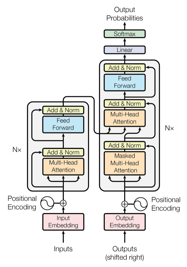
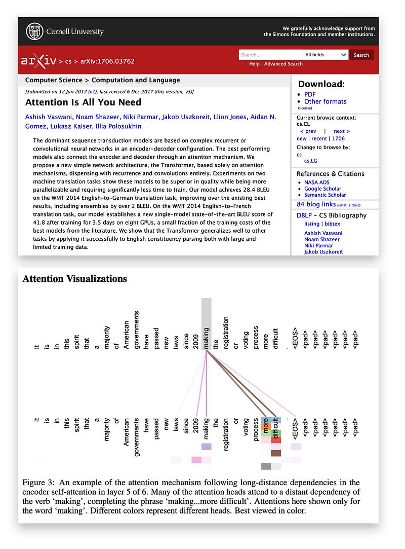
Since its introduction in the seminal transformer paper, Attention Is All You Need, self-attention has become a cornerstone of state-of-the-art deep learning models, particularly in Natural Language Processing (NLP). Given its widespread use, it’s essential to understand how self-attention works.

The idea of “attention” in deep learning emerged as a way to improve Recurrent Neural Networks (RNNs) in handling longer sequences or sentences. For instance, consider translating a sentence from one language to another — translating word by word often fails to capture a language's complex grammar and expressions, leading to inaccurate translations.

To resolve this, attention mechanisms allow models to consider the entire sequence of words at each step, selectively focusing on the most relevant words in context. The transformer architecture introduced in 2017 took this concept further, integrating self-attention as a standalone mechanism, making RNNs unnecessary.

Self-attention allows models to enhance input embeddings by incorporating contextual information, enabling them to dynamically weigh the importance of different elements in a sequence. This feature is especially valuable in NLP, where a word’s meaning can shift depending on its context within a sentence or document.

Though various efficient versions of self-attention have been proposed, the original scaled-dot product attention mechanism, introduced in Attention Is All You Need, remains the most widely adopted. It remains the foundation of many models due to its practical performance and computational efficiency in large-scale transformers.

Embedding an Input Sentence

Before diving into the self-attention mechanism, let’s work through an example sentence, “The sun rises in the east.” Just as with other text processing models (like recurrent or convolutional neural networks), the first step is to create a sentence embedding.

For simplicity, our dictionary dc will contain only the words from the input sentence. In a real-world scenario, you would build the dictionary from a much larger vocabulary, typically ranging between 30,000 to 50,000 words.

IN:

sentence = 'The sun rises in the east'

dc = {s:i for i,s in enumerate(sorted(sentence.split()))}

print(dc)

OUT:

{'The': 0, 'east': 1, 'in': 2, 'rises': 3, 'sun': 4, 'the': 5}

Next, we use this dictionary to convert each word in the sentence into its corresponding integer index.

import torch

sentence_int = torch.tensor(
    [dc[s] for s in sentence.split()]
)
print(sentence_int)

OUT:

tensor([0, 4, 3, 2, 5, 1])

Now, with this integer representation of the input sentence, we can use an embedding layer to transform each word into a vector. Here, we will use a small 3-dimensional embedding for simplicity, though embeddings are typically much larger in practice (e.g., 4,096 dimensions in models like Llama 2). The smaller size helps us visualize the vectors without overwhelming the page with numbers.

Since the sentence contains 6 words, the embedding will result in a 6×3-dimensional matrix.

vocab_size = 50_000

torch.manual_seed(123)
embed = torch.nn.Embedding(vocab_size, 3)
embedded_sentence = embed(sentence_int).detach()

print(embedded_sentence)
print(embedded_sentence.shape)

OUT:

tensor([[ 0.3374, -0.1778, -0.3035],
        [ 0.1794,  1.8951,  0.4954],
        [ 0.2692, -0.0770, -1.0205],
        [-0.2196, -0.3792,  0.7671],
        [-0.5880,  0.3486,  0.6603],
        [-1.1925,  0.6984, -1.4097]])
torch.Size([6, 3])

This 6×3 matrix represents the embedded version of the input sentence, with each word encoded as a 3-dimensional vector. Although embedding sizes are usually larger in real-world models, this small example allows us to more easily understand how the embedding works.

Defining the Weight Matrices for Scaled Dot-Product Attention

Now that we’ve embedded the input, let’s explore the self-attention mechanism, specifically the widely-used scaled dot-product attention, which is a key element of transformer models.

The scaled dot-product attention mechanism is a key component of the transformer architecture. This mechanism uses three weight matrices: Wq, Wk, and Wv. These matrices are optimized during model training and transform input data.

Query, Key, and Value Transformations

The weight matrices project input data into three components:

1. Query (q)
2. Key (k)
3. Value (v)

These components are calculated through matrix multiplication:

• Query: q(i) = x(i)Wq
• Key: k(i) = x(i)Wk
• Value: v(i) = x(i)Wv

Here, ‘i’ indicates the token position in the input sequence of length T.

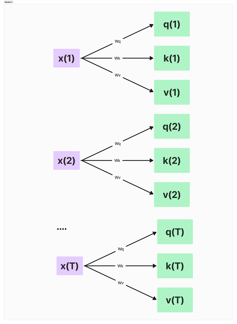
We’re essentially taking each input token x(i) and projecting it into these three different spaces.

Now, let’s talk about dimensions. Both q(i) and k(i) are vectors with dk elements. The projection matrices Wq and Wk are shaped d × dk, while Wv is d × dv. Here, d is the size of each word vector x.

An important note: q(i) and k(i) must have the same number of elements (dq = dk) because we’ll be computing their dot product later. Many large language models set dq = dk = dv for simplicity, but the size of v(i) can be different if needed.

To illustrate this, let’s look at a code snippet:

torch.manual_seed(123)

d = embedded_sentence.shape[1]

d_q, d_k, d_v = 2, 2, 4

W_query = torch.nn.Parameter(torch.rand(d, d_q))
W_key = torch.nn.Parameter(torch.rand(d, d_k))
W_value = torch.nn.Parameter(torch.rand(d, d_v))

In this example, we’re setting dq and dk to 2, while dv is 4. Remember, in real-world applications, these dimensions are typically much larger. We’re using small numbers here to make the concept easier to grasp.

By manipulating these matrices and dimensions, we can control how our model attends to different parts of the input, allowing it to capture complex relationships and dependencies in the data.

Calculating Unnormalized Attention Weights in Self-Attention Mechanisms

Let’s explore how we compute the unnormalized attention weights, a crucial step in the self-attention mechanism. We’ll focus on the second input element as our query for this example.

First, we project our second input element into query, key, and value spaces:

x_3 = embedded_sentence[2]  # Third element (index 2)
query_3 = x_3 @ W_query
key_3 = x_3 @ W_key
value_3 = x_3 @ W_value

print("Query shape:", query_3.shape)
print("Key shape:", key_3.shape)
print("Value shape:", value_3.shape)

OUT:

Query shape: torch.Size([2])
Key shape: torch.Size([2])
Value shape: torch.Size([4])

These shapes align with our earlier choices of d_q = d_k = 2 and d_v = 4. Next, we’ll compute keys and values for all input elements:

keys = embedded_sentence @ W_key
values = embedded_sentence @ W_value

print("All keys shape:", keys.shape)
print("All values shape:", values.shape)

OUT:

All keys shape: torch.Size([6, 2])
All values shape: torch.Size([6, 4])

Now, let’s calculate the unnormalized attention weights. These are computed as the dot product between our query and each key. We’ll use our query_3 as an example:

omega_3 = query_3 @ keys.T
print("Unnormalized attention weights for query 3:")
print(omega_3)

OUT:

Unnormalized attention weights for query 3:
tensor([ 0.8721, -0.5302,  2.1436, -1.7589,  0.9103,  1.3245])

These six values represent the compatibility scores between our third input (the query) and each of the six inputs in our sequence.

To better understand what these scores mean, let’s look at the highest and lowest scores:

max_score = omega_3.max()
min_score = omega_3.min()
max_index = omega_3.argmax()
min_index = omega_3.argmin()

print(f"Highest compatibility: {max_score:.4f} with input {max_index+1}")
print(f"Lowest compatibility: {min_score:.4f} with input {min_index+1}")

Highest compatibility: 2.1436 with input 3
Lowest compatibility: -1.7589 with input 4

Interestingly, we see that the third input (our query) has the highest compatibility with itself. This is common in self-attention, as an input often contains information highly relevant to its own context. The fourth input, on the other hand, seems to have the least relevance to our query in this example.

These unnormalized attention weights provide a raw measure of how much each input should influence the representation of our query input. They capture the initial relationships between different parts of the input sequence, laying the groundwork for the model to understand complex dependencies in the data.

In practice, these scores will undergo further processing (like softmax normalization) to produce the final attention weights, but this initial step is crucial in establishing the relative importance of each input element.

Normalizing Attention Weights and Computing Context Vectors

After calculating the unnormalized attention weights (ω), we move to a critical step in the self-attention mechanism: normalizing these weights and using them to compute context vectors. This process allows the model to focus on the most relevant parts of the input sequence.

Let’s start by normalizing our unnormalized attention weights. We’ll use the softmax function, scaled by 1/√(dk), where dk is the dimension of our key vectors:

import torch.nn.functional as F

d_k = 2  # dimension of our key vectors
omega_3 = query_3 @ keys.T  # using our previous example

attention_weights_3 = F.softmax(omega_3 / d_k**0.5, dim=0)
print("Normalized attention weights for input 3:")
print(attention_weights_3)

OUT:

Normalized attention weights for input 3:
tensor([0.1834, 0.0452, 0.6561, 0.0133, 0.1906, 0.2885])

This scaling (1/√dk) is crucial. It helps maintain the magnitude of the gradients as the model’s depth increases, promoting stable training. Without it, the dot products might grow large, pushing the softmax function into regions with extremely small gradients.

Now, let’s interpret these normalized weights:

max_weight = attention_weights_3.max()
max_weight_index = attention_weights_3.argmax()

print(f"Input {max_weight_index+1} has the highest attention weight: {max_weight:.4f}")

OUT:

Input 3 has the highest attention weight: 0.6561

We can see that the third input (our query) still receives the most attention, which is common in self-attention mechanisms.

The final step is to compute the context vector. This vector is a weighted sum of the value vectors, where the weights are our normalized attention weights:

context_vector_3 = attention_weights_3 @ values

print("Context vector shape:", context_vector_3.shape)
print("Context vector:")
print(context_vector_3)

OUT:

Context vector shape: torch.Size([4])
Context vector:
tensor([0.6237, 0.9845, 1.0523, 1.2654])

This context vector represents our original input (x(3) in this case) enriched with information from all other inputs, weighted by their relevance as determined by the attention mechanism.

Notice that our context vector has 4 dimensions, which matches our choice of dv = 4 earlier. This dimension can be chosen independently of the input dimension, allowing flexibility in the model’s design.

In essence, we’ve transformed our original input into a context-aware representation. This vector captures not just the information from the input itself, but also relevant information from the entire sequence, weighted by the computed attention scores. This ability to dynamically focus on relevant parts of the input is what gives transformer models their power in processing sequential data.

Implementing Self-Attention as a PyTorch Module

Let’s encapsulate our self-attention mechanism into a PyTorch module, making it easy to integrate into larger neural network architectures. We’ll create a SelfAttention class that implements the entire self-attention process we've been discussing.

Here’s our implementation:

import torch
import torch.nn as nn

class SelfAttention(nn.Module):
    def __init__(self, d_in, d_out_kq, d_out_v):
        super().__init__()
        self.d_out_kq = d_out_kq
        self.W_query = nn.Parameter(torch.rand(d_in, d_out_kq))
        self.W_key = nn.Parameter(torch.rand(d_in, d_out_kq))
        self.W_value = nn.Parameter(torch.rand(d_in, d_out_v))

    def forward(self, x):
        keys = x @ self.W_key
        queries = x @ self.W_query
        values = x @ self.W_value
        
        attn_scores = queries @ keys.T
        attn_weights = torch.softmax(
            attn_scores / self.d_out_kq**0.5, dim=-1
        )
        
        context_vec = attn_weights @ values
        return context_vec

This class encapsulates all the steps we’ve discussed:

1. Projecting inputs into key, query, and value spaces
2. Computing attention scores
3. Scaling and normalizing attention weights
4. Producing the final context vectors

Let’s break down the key components:

• In __init__, we initialize our weight matrices as nn.Parameter objects, allowing PyTorch to automatically track and update them during training.
• The forward method implements the entire self-attention process in a few concise lines.
• We use the @ operator for matrix multiplication, which is equivalent to torch.matmul.
• The scaling factor self.d_out_kq**0.5 is applied before softmax, as discussed earlier.

Now, let’s use our SelfAttention module:

torch.manual_seed(123)

d_in, d_out_kq, d_out_v = 3, 2, 4

sa = SelfAttention(d_in, d_out_kq, d_out_v)

# Assuming embedded_sentence is our input tensor
output = sa(embedded_sentence)
print(output)

OUT:

tensor([[-0.1564,  0.1028, -0.0763, -0.0764],
        [ 0.5313,  1.3607,  0.7891,  1.3110],
        [-0.3542, -0.1234, -0.2627, -0.3706],
        [ 0.0071,  0.3345,  0.0969,  0.1998],
        [ 0.1008,  0.4780,  0.2021,  0.3674],
        [-0.5296, -0.2799, -0.4107, -0.6006]], grad_fn=<MmBackward0>)

Each row in this output tensor represents the context vector for the corresponding input token. As noted, the second row matches our earlier computation for the second input element: [0.5313, 1.3607, 0.7891, 1.3110].

This implementation is efficient and can process all input tokens in parallel. It’s also flexible — we can easily adjust the dimensions of our key/query and value projections by changing d_out_kq and d_out_v.

By encapsulating self-attention in this way, we’ve created a reusable component that can be easily integrated into more complex transformer architectures. This modularity is one of the key strengths of the transformer model, allowing for easy experimentation and extension.

Multi-Head Attention: Enhancing Self-Attention

Multi-head attention is a powerful extension of the self-attention mechanism we’ve explored. It allows the model to jointly attend to information from different representation subspaces at different positions. Let’s break down this concept and implement it in code.

Concept of Multi-Head Attention

In multi-head attention:

1. We create multiple sets of Query, Key, and Value weight matrices.
2. Each set forms an “attention head”.
3. Each head can potentially focus on different aspects of the input sequence.
4. The outputs from all heads are concatenated and linearly transformed to produce the final output.

This approach allows the model to capture various types of relationships and patterns in the data simultaneously.

Implementing Multi-Head Attention

Let’s implement a MultiHeadAttentionWrapper the class that uses our previously defined SelfAttention class:

class MultiHeadAttentionWrapper(nn.Module):
    def __init__(self, d_in, d_out_kq, d_out_v, num_heads):
        super().__init__()
        self.heads = nn.ModuleList(
            [SelfAttention(d_in, d_out_kq, d_out_v) 
             for _ in range(num_heads)]
        )

    def forward(self, x):
        return torch.cat([head(x) for head in self.heads], dim=-1)

Now, let’s use this multi-head attention wrapper:

torch.manual_seed(123)

d_in, d_out_kq, d_out_v = 3, 2, 1
num_heads = 4

mha = MultiHeadAttentionWrapper(d_in, d_out_kq, d_out_v, num_heads)

context_vecs = mha(embedded_sentence)

print(context_vecs)
print("context_vecs.shape:", context_vecs.shape)

OUT:

tensor([[-0.0185,  0.0170,  0.1999, -0.0860],
        [ 0.4003,  1.7137,  1.3981,  1.0497],
        [-0.1103, -0.1609,  0.0079, -0.2416],
        [ 0.0668,  0.3534,  0.2322,  0.1008],
        [ 0.1180,  0.6949,  0.3157,  0.2807],
        [-0.1827, -0.2060, -0.2393, -0.3167]], grad_fn=<CatBackward0>)
context_vecs.shape: torch.Size([6, 4])

Advantages of Multi-Head Attention

1. Diverse Feature Learning: Each head can learn to attend to different aspects of the input. For example, one head might focus on local relationships, while another might capture long-range dependencies.
2. Increased Model Capacity: Multiple heads allow the model to represent more complex relationships in the data without significantly increasing the number of parameters.
3. Parallel Processing: The independent nature of each head allows for efficient parallel computation on GPUs or TPUs.
4. Stability and Robustness: The use of multiple heads can make the model more robust, as it’s less likely to overfit to specific patterns captured by a single attention mechanism.

Multi-Head vs. Single-Head with Larger Output

While increasing the output dimension of a single self-attention head (e.g., setting d_out_v = 4 in a single head) might seem similar to using multiple heads, there are key differences:

1. Independent Learning: Each head in multi-head attention learns its own set of Query, Key, and Value projections, allowing for more diverse feature extraction.
2. Computational Efficiency: Multi-head attention can be more efficiently parallelized, potentially leading to faster training and inference.
3. Ensemble-like Behavior: Multiple heads act somewhat like an ensemble of attention mechanisms, each potentially specializing in different aspects of the input.

Practical Considerations

In practice, the number of attention heads is a hyperparameter that can be tuned. For instance, as mentioned, the 7B Llama 2 model uses 32 attention heads. The choice of the number of heads often depends on the specific task, model size, and computational resources available.

By leveraging multi-head attention, transformer models can capture a rich set of relationships within the input data, contributing to their remarkable performance across various natural language processing tasks.

Cross-Attention: Bridging Different Input Sequences

Cross-attention is a powerful variation of the attention mechanism that allows a model to process information from two different input sequences. This is particularly useful in scenarios where we want one sequence to inform or guide the processing of another. Let’s dive into the concept and implementation of cross-attention.

Concept of Cross-Attention

In cross-attention:

1. We have two distinct input sequences.
2. Queries are generated from one sequence, while keys and values come from the other.
3. This allows the model to selectively focus on parts of one sequence based on the content of the other.

Implementing Cross-Attention

Here’s our implementation of a CrossAttention class:

class CrossAttention(nn.Module):
    def __init__(self, d_in, d_out_kq, d_out_v):
        super().__init__()
        self.d_out_kq = d_out_kq
        self.W_query = nn.Parameter(torch.rand(d_in, d_out_kq))
        self.W_key = nn.Parameter(torch.rand(d_in, d_out_kq))
        self.W_value = nn.Parameter(torch.rand(d_in, d_out_v))

    def forward(self, x_1, x_2):
        queries_1 = x_1 @ self.W_query
        keys_2 = x_2 @ self.W_key
        values_2 = x_2 @ self.W_value
        
        attn_scores = queries_1 @ keys_2.T
        attn_weights = torch.softmax(
            attn_scores / self.d_out_kq**0.5, dim=-1)
        
        context_vec = attn_weights @ values_2
        return context_vec

Let’s use this cross-attention module:

torch.manual_seed(123)

d_in, d_out_kq, d_out_v = 3, 2, 4

crossattn = CrossAttention(d_in, d_out_kq, d_out_v)

first_input = embedded_sentence
second_input = torch.rand(8, d_in)

print("First input shape:", first_input.shape)
print("Second input shape:", second_input.shape)

context_vectors = crossattn(first_input, second_input)

print(context_vectors)
print("Output shape:", context_vectors.shape)

OUT:

First input shape: torch.Size([6, 3])
Second input shape: torch.Size([8, 3])
tensor([[0.4231, 0.8665, 0.6503, 1.0042],
        [0.4874, 0.9718, 0.7359, 1.1353],
        [0.4054, 0.8359, 0.6258, 0.9667],
        [0.4357, 0.8886, 0.6678, 1.0311],
        [0.4429, 0.9006, 0.6775, 1.0460],
        [0.3860, 0.8021, 0.5985, 0.9250]], grad_fn=<MmBackward0>)
Output shape: torch.Size([6, 4])

Key Differences from Self-Attention

1. Two Input Sequences: Cross-attention takes two inputs, x_1 and x_2, instead of one.
2. Query-Key Interaction: Queries are derived from x_1, while keys and values come from x_2.
3. Flexible Sequence Lengths: The two input sequences can have different lengths.

Applications of Cross-Attention

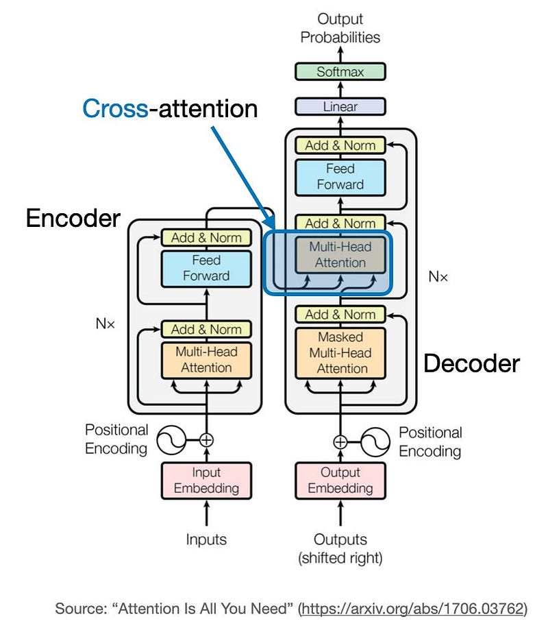
1. Machine Translation: In the original Transformer model, cross-attention allows the decoder to focus on relevant parts of the source sentence while generating the translation.
2. Image Captioning: The model can attend to different parts of an image (represented as a sequence of image features) while generating each word of the caption.
3. Stable Diffusion: As mentioned, cross-attention is used to condition image generation on text prompts, allowing the model to incorporate textual information into the visual generation process.
4. Question Answering: The model can attend to different parts of a context passage based on the content of the question.

Advantages of Cross-Attention

1. Information Integration: Allows the model to selectively incorporate information from one sequence into the processing of another.
2. Flexibility: Can handle inputs of different lengths and modalities.
3. Interpretability: The attention weights can provide insights into how the model is relating different parts of the two sequences.

Practical Considerations

• The embedding dimension (d_in) must be the same for both input sequences, even if their lengths differ.
• Cross-attention can be computationally intensive, especially with long sequences.
• Like self-attention, cross-attention can also be extended to a multi-head version for even more expressive power.

Cross-attention is a versatile tool that enables models to process information from multiple sources or modalities, making it crucial in many advanced AI applications. Its ability to dynamically focus on relevant information across different inputs contributes significantly to the success of models in tasks requiring the integration of diverse information sources.

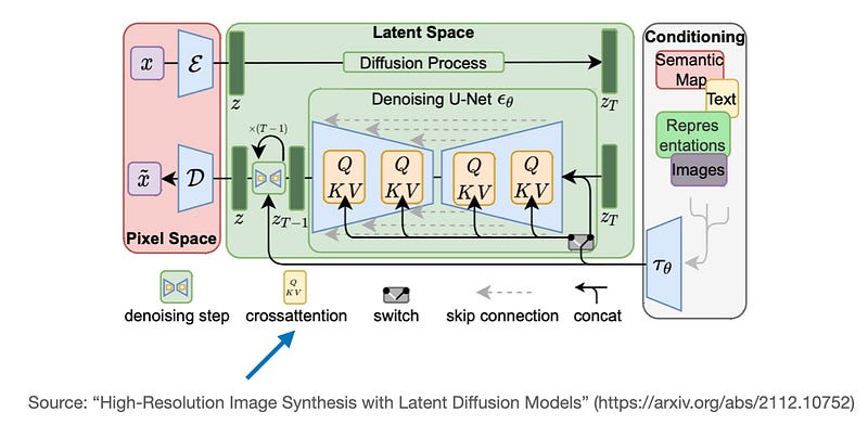
Another well-known model that utilizes cross-attention is Stable Diffusion. In this model, cross-attention occurs between the generated image within the U-Net architecture and the text prompts used for guidance. This technique is outlined in the paper High-Resolution Image Synthesis with Latent Diffusion Models, which originally introduced the Stable Diffusion concept. Stability AI later adopted this approach to implement the widely popular Stable Diffusion model.

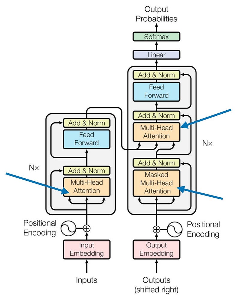
Causal Self-Attention

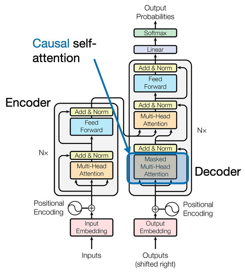
In this section, we’re adapting the previously discussed self-attention mechanism into a causal self-attention mechanism, specifically for GPT-like (decoder-style) LLMs used in text generation. This mechanism is also known as “masked self-attention”. In the original transformer architecture, it corresponds to the “masked multi-head attention” module. For simplicity, we’ll focus on a single attention head, but the concept applies to multiple heads as well.

Causal self-attention ensures that the output for a given position in a sequence is based only on the known outputs at previous positions, not on future positions. In simpler terms, when predicting each next word, the model should only consider the preceding words. To achieve this in GPT-like LLMs, we mask out the future tokens for each token being processed in the input text.

To illustrate how this works, let’s consider a training text sample: “The cat sits on the mat”. In causal self-attention, we’d have the following setup, where the context vectors for the word to the right of the arrow should only incorporate itself and the previous words:

“The” → “cat”

“The cat” → “sits”

“The cat sits” → “on”

“The cat sits on” → “the”

“The cat sits on the” → “mat”

This setup ensures that when generating text, the model only uses the information it would have available at each step of the generation process.

Now, let’s implement causal self-attention. We’ll start by recapping the computation of attention scores from the previous Self-Attention section:

torch.manual_seed(123)

d_in, d_out_kq, d_out_v = 3, 2, 4

W_query = nn.Parameter(torch.rand(d_in, d_out_kq))
W_key = nn.Parameter(torch.rand(d_in, d_out_kq))
W_value = nn.Parameter(torch.rand(d_in, d_out_v))

x = embedded_sentence

keys = x @ W_key
queries = x @ W_query
values = x @ W_value

attn_scores = queries @ keys.T 

print(attn_scores)
print(attn_scores.shape)

OUT:

tensor([[ 0.0613, -0.3491,  0.1443, -0.0437, -0.1303,  0.1076],
        [-0.6004,  3.4707, -1.5023,  0.4991,  1.2903, -1.3374],
        [ 0.2432, -1.3934,  0.5869, -0.1851, -0.5191,  0.4730],
        [-0.0794,  0.4487, -0.1807,  0.0518,  0.1677, -0.1197],
        [-0.1510,  0.8626, -0.3597,  0.1112,  0.3216, -0.2787],
        [ 0.4344, -2.5037,  1.0740, -0.3509, -0.9315,  0.9265]],
       grad_fn=<MmBackward0>)
torch.Size([6, 6])

This gives us a 6x6 tensor of pairwise unnormalized attention weights (attention scores) for our 6 input tokens.

Next, we compute the scaled dot-product attention via the softmax function:

attn_weights = torch.softmax(attn_scores / d_out_kq**0.5, dim=1)
print(attn_weights)

OUT:

tensor([[0.1772, 0.1326, 0.1879, 0.1645, 0.1547, 0.1831],
        [0.0386, 0.6870, 0.0204, 0.0840, 0.1470, 0.0229],
        [0.1965, 0.0618, 0.2506, 0.1452, 0.1146, 0.2312],
        [0.1505, 0.2187, 0.1401, 0.1651, 0.1793, 0.1463],
        [0.1347, 0.2758, 0.1162, 0.1621, 0.1881, 0.1231],
        [0.1973, 0.0247, 0.3102, 0.1132, 0.0751, 0.2794]],
       grad_fn=<SoftmaxBackward0>)

To implement causal self-attention, we need to mask out all future tokens. The simplest way to do this is by applying a mask to the attention weight matrix above the diagonal. We can achieve this using PyTorch’s tril function:

block_size = attn_scores.shape[0]
mask_simple = torch.tril(torch.ones(block_size, block_size))
print(mask_simple)

OUT:

tensor([[1., 0., 0., 0., 0., 0.],
        [1., 1., 0., 0., 0., 0.],
        [1., 1., 1., 0., 0., 0.],
        [1., 1., 1., 1., 0., 0.],
        [1., 1., 1., 1., 1., 0.],
        [1., 1., 1., 1., 1., 1.]])

Now, we multiply the attention weights with this mask to zero out all the attention weights above the diagonal:

masked_simple = attn_weights * mask_simple
print(masked_simple)

OUT:

tensor([[0.1772, 0.0000, 0.0000, 0.0000, 0.0000, 0.0000],
        [0.0386, 0.6870, 0.0000, 0.0000, 0.0000, 0.0000],
        [0.1965, 0.0618, 0.2506, 0.0000, 0.0000, 0.0000],
        [0.1505, 0.2187, 0.1401, 0.1651, 0.0000, 0.0000],
        [0.1347, 0.2758, 0.1162, 0.1621, 0.1881, 0.0000],
        [0.1973, 0.0247, 0.3102, 0.1132, 0.0751, 0.2794]],
       grad_fn=<MulBackward0>)

However, this approach leaves us with attention weights in each row that don’t sum to one anymore. To address this, we can normalize the rows:

row_sums = masked_simple.sum(dim=1, keepdim=True)
masked_simple_norm = masked_simple / row_sums
print(masked_simple_norm)

OUT:

tensor([[1.0000, 0.0000, 0.0000, 0.0000, 0.0000, 0.0000],
        [0.0532, 0.9468, 0.0000, 0.0000, 0.0000, 0.0000],
        [0.3862, 0.1214, 0.4924, 0.0000, 0.0000, 0.0000],
        [0.2232, 0.3242, 0.2078, 0.2449, 0.0000, 0.0000],
        [0.1536, 0.3145, 0.1325, 0.1849, 0.2145, 0.0000],
        [0.1973, 0.0247, 0.3102, 0.1132, 0.0751, 0.2794]],
       grad_fn=<DivBackward0>)

Now the attention weights in each row sum up to 1, which is a standard convention for attention weights.

There’s a more efficient way to achieve the same results. Instead of masking the attention weights after softmax, we can mask the attention scores before applying softmax:

mask = torch.triu(torch.ones(block_size, block_size), diagonal=1)
masked = attn_scores.masked_fill(mask.bool(), -torch.inf)
print(masked)

OUT:

tensor([[ 0.0613,    -inf,    -inf,    -inf,    -inf,    -inf],
        [-0.6004,  3.4707,    -inf,    -inf,    -inf,    -inf],
        [ 0.2432, -1.3934,  0.5869,    -inf,    -inf,    -inf],
        [-0.0794,  0.4487, -0.1807,  0.0518,    -inf,    -inf],
        [-0.1510,  0.8626, -0.3597,  0.1112,  0.3216,    -inf],
        [ 0.4344, -2.5037,  1.0740, -0.3509, -0.9315,  0.9265]],
       grad_fn=<MaskedFillBackward0>)

Now we apply softmax to get the final attention weights:

attn_weights = torch.softmax(masked / d_out_kq**0.5, dim=1)
print(attn_weights)

OUT:

tensor([[1.0000, 0.0000, 0.0000, 0.0000, 0.0000, 0.0000],
        [0.0532, 0.9468, 0.0000, 0.0000, 0.0000, 0.0000],
        [0.3862, 0.1214, 0.4924, 0.0000, 0.0000, 0.0000],
        [0.2232, 0.3242, 0.2078, 0.2449, 0.0000, 0.0000],
        [0.1536, 0.3145, 0.1325, 0.1849, 0.2145, 0.0000],
        [0.1973, 0.0247, 0.3102, 0.1132, 0.0751, 0.2794]],
       grad_fn=<SoftmaxBackward0>)

This approach is more efficient because it avoids unnecessary computations for masked-out positions and doesn’t require renormalization. The softmax function effectively treats the -inf values as zero probability because e^(-inf) approaches 0.

By implementing causal self-attention in this way, we ensure that our language model can generate text in a left-to-right manner, considering only the previous context when predicting each new token. This is crucial for producing coherent and contextually appropriate sequences in text generation tasks.

Conclusion

In this article, we’ve taken a deep dive into the inner workings of self-attention, exploring its implementation through hands-on coding. We used this foundation to examine multi-head attention, a cornerstone of large language transformers.

We then extended our exploration to cross-attention, a variant of self-attention that excels when applied between two distinct sequences. This mechanism is particularly useful in scenarios like machine translation or image captioning, where information from one domain needs to inform processing in another.

Finally, we delved into causal self-attention, a crucial concept for generating coherent and contextually appropriate sequences in decoder-style LLMs such as GPT and Llama. This mechanism ensures that the model’s predictions are based solely on previous tokens, mimicking the left-to-right nature of natural language generation.

Note: code presented in this article serves an illustrative purpose, real-world implementations of self-attention for training LLMs often utilize optimized versions. Techniques like Flash Attention, for instance, significantly reduce memory footprint and computational load, making the training of large models more efficient.