Unlocking the Power of Linear Regression — Diving Deeper into the World of Predictive Modeling

Linear regression is a fundamental statistical and machine learning technique used for modelling the relationship between a dependent variable (target) and one or more independent variables (features). It assumes a linear relationship between the variables, where changes in the independent variables are linearly related to changes in the dependent variable.

There are many articles online the describe how/what Linear regression works/is but there is little information about the maths behind the scene. Most of them give you some pre-implemented library to run a linear regression algorithm on a pre-generated data set. You are probably still not sure what it is even you are able to program it. In this article, I am going to talk about the mathematics about linear regression and its intuition. In the end, I will give a real dataset example and take you step by step about how to improve the prediction by training the model differently.

What is regression?

In the context of linear regression, the term “regression” refers to the process of finding a line or curve that best fits a set of data points. In other words, Regressing Towards the Mean. It is a statistical concept that describes the tendency of variables to move towards their average values over time or with repeated measurements. It’s important to consider regression when interpreting data and making predictions, as it can help avoid over-interpreting extreme results or assuming that exceptional events will always repeat themselves.

Here are several examples to illustrate the meaning of “regression” in different contexts:

• Height and Parental Height Observation: Children of exceptionally tall parents tend to be shorter than their parents, while children of exceptionally short parents tend to be taller. Regression: This demonstrates regression towards the mean, as heights tend to “regress” or move back towards an average value over generations.
• Test Scores and Study Hours Scenario: A student scores very high on a test after studying for a long time. On the next test, they don’t study as much and their score drops. Regression: This is a regression towards the mean. It’s likely that the student’s first score was a bit above their typical performance, and the second score was a bit below, both moving closer to their average ability.
• Sports Performance Scenario: A basketball player has an exceptional game, scoring far above their average. In the following game, they score closer to their usual average. Regression: This is also regression towards the mean. It’s unlikely that the player will consistently score at their peak level every game, so their performance tends to regress towards their average.
• Financial Markets Observation: A stock that has experienced a sharp increase in price often sees a period of decline or stabilization afterward. Regression: This is often attributed to regression to the mean, as prices tend to revert back to their longer-term average values after extreme fluctuations.
• Medical Research Scenario: A new drug shows promising results in an initial trial. However, in a larger follow-up trial, the results are less impressive. Regression: This could be due to regression to the mean. The initial trial might have included participants who experienced a more beneficial response than average, while the larger trial included a more representative sample.

The Mathematics (hypothesis function)

Linear regression is a statistical method used to model the relationship between a dependent variable (y) and one or more independent variables (x). It assumes a linear relationship, meaning that the change in y is proportional to the change in x. Let’s start work on the maths part of this algorithm from an example.

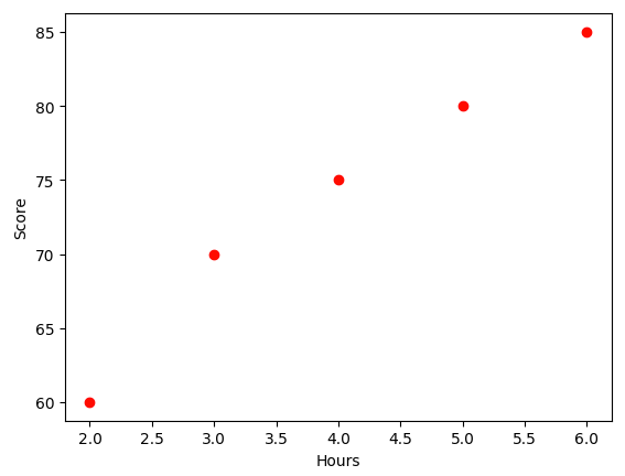
Suppose we want to understand the relationship between the number of hours students study and their exam scores. We hypothesize that there’s a linear relationship between these two variables: as study hours increase, exam scores also increase.

Data: We collect data from a sample of students, recording their study hours and corresponding exam scores. It only have one independent variable (study hours) so it is called simple linear regression.

The data is very simple, it has one parameter which is Study Hours (x) and Exam Score (y) . Below is the plot of this two values:

Objective: We aim to build a linear regression model to predict exam scores based on study hours. You want to find the values of ⍺​ and ⍬​ that minimize the Mean Squared Error (MSE), the cost function in this regression model, to obtain the best-fitting line that represents the relationship between study hour and exam score. In other words, we need to find a line shown in the above diagram to make every point is close to that line. The function of that line is cost function.

Linear Regression Model: The simple linear regression model (it is also called hypothesis function) sis represented as:

h(x) = ⍺x + ⍬

Where:

• h(x) = Exam Score (dependent variable), the hypothesis function
• x = Study Hours (independent variable)
• ⍺ = slop
• ⍬ = h(x)-intercept

Cost Function

In linear regression, the cost function, also known as the loss function or objective function, quantifies the difference between the predicted values from the model and the actual values in the training data. The goal is to minimise this cost function to find the best-fitting line (or hyperplane in multiple dimensions) that represents the relationship between the independent variables and the dependent variable.

For simple linear regression with one independent variable, the cost function is typically the Mean Squared Error (MSE) or the Sum of Squared Errors (SSE). It measures the average squared difference between the observed values (actual values) and the predicted values from the hypothesis function.

The formula of a cost function J is (we use J to represent the cost function):

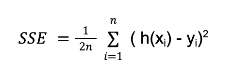
Where:

• y: Actual value of the dependent variable for the x data point.
• h(x): Predicted value of the dependent variable for the x data point (obtained from the regression model above).
• n: Total number of data points.

This equation can be used to get the distance between each predicted value and the actual value. The job is to find the i that makes SSE minimum.

why does cost function in linear regression algorithm have square?

There are several reasons for using the square of the errors in the cost function:

1. Positive and Negative Errors Squaring the errors ensures that both positive and negative deviations from the actual values contribute to the overall error. Without squaring, positive and negative errors could cancel each other out, resulting in a potentially misleading assessment of the model’s performance.
2. Penalizing Larger Errors Squaring amplifies the effect of larger errors. By penalizing larger errors more severely, the model is incentivized to minimize the impact of outliers or extreme deviations, leading to a more robust fit to the majority of the data points.
3. Mathematical Simplicity and Continuity Squared errors lead to a differentiable and convex cost function, facilitating efficient optimization techniques, such as gradient descent, to find the optimal parameters for the hypothesis function. The use of squares results in a smooth, continuous function that is well-suited for optimization algorithms.
4. Mean Squared Error Interpretation The Mean Squared Error (MSE), which is the average of the squared errors, provides a measure of the average magnitude of errors between the predicted and actual values. The squared units (e.g., squared meters, squared dollars) can be interpreted in the context of the original dependent variable, offering a meaningful assessment of the model’s predictive accuracy.
5. Statistical Assumptions In the context of ordinary least squares (OLS) linear regression, minimizing the sum of squared residuals (errors) corresponds to maximizing the likelihood of the observed data under certain assumptions, such as normally distributed errors with constant variance (homoscedasticity). The squared residuals align with the underlying statistical framework and assumptions of the hypothesis function.

Once you understand Linear regression model and Cost function, the final part is to find the right prediction model to predict the exam score based on study hours. The goal is to find the parameters ⍺, ⍬ for the formula y = ⍺x + ⍬ that to make the cost function as small as possible. Why do we need to make it small? Let randomly pick up some values for ⍺ to plot the prediction line. To make it simple, let make ⍬ as 0 for now.

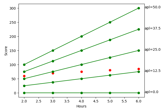
The above diagram includes the original 5 red points from our dataset plus 5 green lines each. Each of the green line is plotted based on a random alpha value from the formula y = ⍺x . As we can see that the two lines (alpha=12.5 and alpha=25.0) are very close to the red points. The cost function mentioned above is to use the formula to find the smallest value which is to find the line that is the closest to the target RED point. The distance between each point on the green line to the RED point is called error. If we put the above 5 alpha value to the cost function, we can get the minimum value is 12.5.

Let me take you through a manual calculaution when using 12.5 as alpha value. The value of x is: 2,3,4,5,6. The y is: 60, 70, 75, 80, 85. The cost function will be:

cost function: 1 / 10 * (12.5 * 2-60)² + (12.5*3–70)² + (12.5 * 4–75)² + (12.5 * 5–80)² + (12.5 * 6–85)² = 331.25

So the 331.25 is the smallest value we get so far. But it could not be the smallest possible value, we only choose a random 5 alpha values in above diagram.

Overfitting & Underfitting

We can tune the alpha value to find the closest line like:

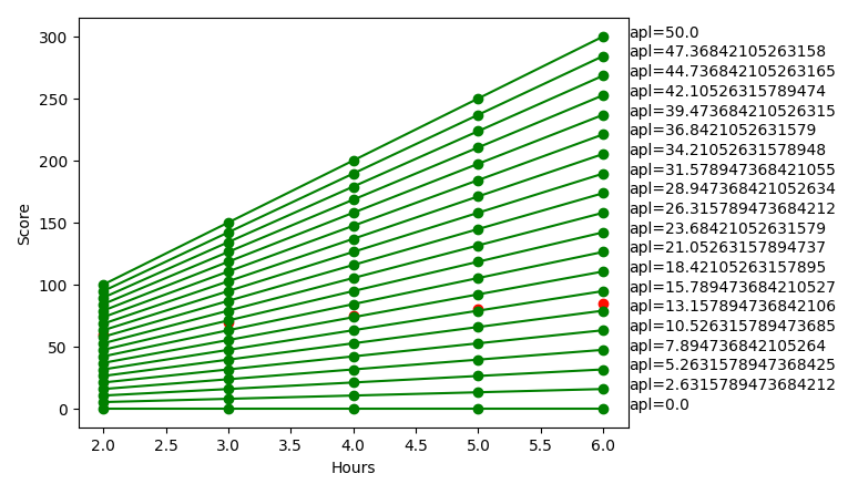
When tuning more values on the cost function for linear regression, several potential problems and challenges may arise, affecting the performance, interpretability, and reliability of the regression model.

Overfitting occurs when a model learns the training data too closely, capturing the noise and random fluctuations in the data rather than the underlying true relationship between variables. As a result, the model may perform well on the training data but generalize poorly to new, unseen data.

Tuning more values on the cost function can lead to complex models that are overly flexible and sensitive to variations in the training data, increasing the risk of overfitting.

Underfitting in linear regression refers to a situation where the model is too simple to capture the underlying patterns and relationships in the data, resulting in a poor fit to both the training data and new, unseen data. It occurs when the model is overly constrained and fails to adequately represent the complexity and variability present in the data, leading to biased and inaccurate predictions.

Multiple dimensional linear regression

The above example is simple since it only has one variable, but in reality there are many parameters we need to deal with. Let’s take another example to see what it looks like when using 2 variables.

The dataset we have is the house price data is shown as below. It has 12 variables and the first one is the house price we are going to predict. I am going to pick two of them Bedrooms and Bathrooms as an example.

I am not going to write the raw formula since it could be very complicated and boring. Understand the formula and manual calculation mentioned from above section is good enough to understand the algorithm. I am going to use python with the machine learning library sklearn.

First, we need to load the dataset as below code. It loads the 5 integer variables into 5 variables, price, area, bedrooms, stories .

from sklearn.linear_model import LinearRegression
import matplotlib.pyplot as plt
import numpy as np
import matplotlib as mpl
import csv
import io
from sklearn.metrics import r2_score
from sklearn.model_selection import train_test_split
import requests

data_url = 'https://raw.githubusercontent.com/zhaoyi0113/machine-learning/master/dataset/housing.csv'

r = requests.get(data_url)
buff = io.StringIO(r.text)
dr = csv.DictReader(buff, delimiter=',')

data_dic = list(dr)
model = LinearRegression()

data_array = np.array(data_dic)
array = np.array([list(d.values()) for d in data_dic])

price, area, bedrooms, bathrooms, stories = (array[:, 0]).astype(float), array[:, 1].astype(float),(array[:, 2]).astype(float), (array[:, 3]).astype(float), (array[:, 4]).astype(float)

Next, let write the code to train the model:

x = np.vstack((bedrooms, bathrooms))
x = x.T

data=x
target=price

data_train, data_test, target_train, target_test = train_test_split(data, target, test_size=0.2, random_state=42)

model = LinearRegression()
model.fit(data_train, target_train)

The code uses LinearRegression model to train and predict the price. It uses the first 80% raws as training dataset and use the last 20% rows to test the trained model.

After trainning the model, we can use the rest 20% data to check how well the model is trainned.

score = model.score(data_test, target_test)
print('score', score)

output: score 0.2605701076698277

The model.score is used to check the model behaviour. The output is 0.26 which means the positive rate is only 26%. It also means it is worse than flipping a coin.

Sometimes, when you start working on training a model, it always gets a very bad result at beginning. It could be caused by various of reasons. For this example, the price is impacted by 12 variables but we only picked 2 of them. It is a lack of training parameters. Next, let me show you how to improve the prediction.

You may think that we can put all variables into the linear regression model but before doing that, let’s review what each of the data variable looks like.

There are two categories of variables,

• Integer: price, area, bedrooms, bathrooms, stories
• String: mainroad, guestroom, basement , hotwater, heating, airconditioning

Let’s look at those integer values first by plotting them in a diagram:

fig, axs = plt.subplots(2,3, figsize = (10,5))

axs[0,0].set_xlabel('Price')
plt1 = sns.boxplot(price, ax = axs[0,0])

axs[0,1].set_xlabel('Area')
plt1 = sns.boxplot(area, ax = axs[0,1])

axs[0,2].set_xlabel('Bedrooms')
plt1 = sns.boxplot(bedrooms, ax = axs[0,2])

axs[1,0].set_xlabel('Bathrooms')
plt1 = sns.boxplot(bathrooms, ax = axs[1, 0])

axs[1,1].set_xlabel('Stories')
plt1 = sns.boxplot(stories, ax = axs[1, 1])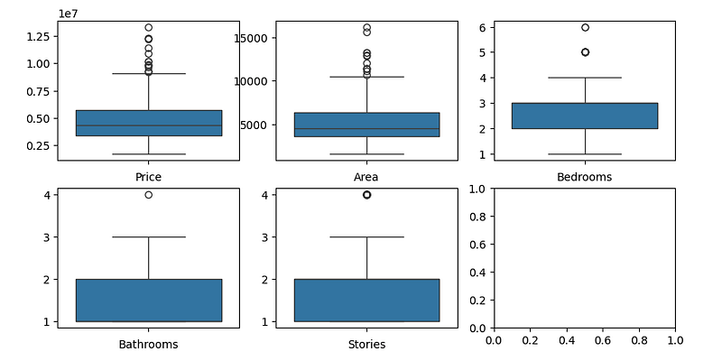

Price and area have considerable outliers. Outliers can pull the line towards themselves, making it less representative of the overall trend in the data. This can lead to inaccurate predictions for new data points, especially those closer to the bulk of the data. We need to normalise them into the same value range.

Normalize X

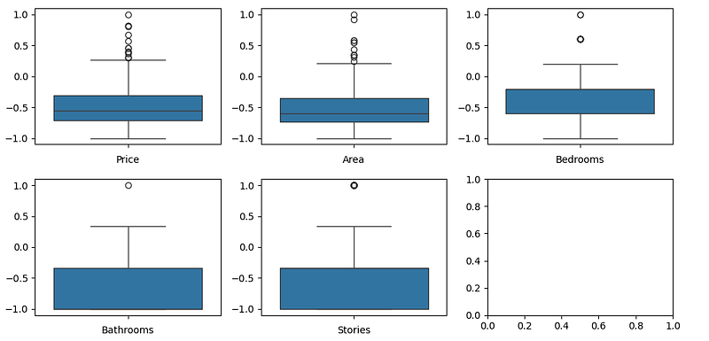
Now, lets normalise X so the values lie between -1 and 1. We do this so we can get all features into a similar range. This assists if we need to plot data, but also gives better linear regression results. We use the following equation and you should see your features now normalised to values similar to figure

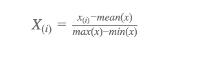
def normalise(arr):
    min_value = np.amin(arr)
    max_value = np.amax(arr)

    # Normalize the array
    normalized_arr = 2 * (arr - min_value) / (max_value - min_value) - 1
    return normalized_arr

nor_price = normalise(price)
nor_bedrooms = normalise(bedrooms)
nor_bathrooms = normalise(bathrooms)
nor_area = normalise(area)
nor_stories = normalise(stories)

After normalise all variables, the plotted diagram will look like:

Let’s try to use above variables to train the model, in order to make it easy to run, I convert the linear regression code into a function which takes unlimited number of variables from its parameter:

def linear_regression(*args):
    target = args[0]
    vars = np.array(args[1:])
    x = np.vstack(vars)
    x = x.T
    
    data=x
    
    data_train, data_test, target_train, target_test = train_test_split(data, target, test_size=0.2, random_state=42)
    
    
    model = LinearRegression()
    model.fit(data_train, target_train)
    
    score = model.score(data_test, target_test)
    print('score', score)
    
    # Create a 3D plot
    fig = plt.figure()
    ax = fig.add_subplot(111, projection='3d')
    
    # Plot the data points
    ax.scatter(x[:, 0], x[:, 1], price)

Then call this function with those normalised values:

linear_regression(nor_price, nor_bedrooms, nor_bathrooms, nor_area, nor_stories)

> score 0.5137585349037066

You might have noticed that the score is increased to 51%.

Don’t forget we also have some unused variables whose value is string. By looking at those data, their values is either yes or no. A common way to convert them to integer is to map yes to 1 and no to 0.

def normalise_string(arr):
    # Define the mapping
    mapping = {'yes': 1, 'no': 0}
    
    # Use the map function to convert the array
    int_arr = list(map(lambda x: mapping[x], arr))
    
    return int_arr

nor_mainroad = normalise_string(mainroad)
nor_guestroom = normalise_string(guestroom)
nor_basement = normalise_string(basement)
nor_hotwaterheating = normalise_string(hotwaterheating)
nor_airconditioning = normalise_string(airconditioning)
nor_prefarea = normalise_string(prefarea)

linear_regression(nor_price, nor_bedrooms, nor_bathrooms, nor_area, nor_stories, nor_parking, nor_mainroad, nor_guestroom, nor_basement, nor_hotwaterheating, nor_airconditioning, nor_prefarea)

> score 0.6437296086614106

As you might have noticed, the score for this version is increased to over 64%.

Conclusion

Linear regression is a versatile and widely used statistical technique for modeling and analyzing relationships between variables, predicting continuous outcomes, and developing interpretable and predictive models based on the underlying linear relationships and patterns in the data. In this article, I have talked about the math theory behind the scene, then give examples about using one variable simple data model and multiple variables model. From the learning result, it shows you how the prediction get improved by using different input parameters.