Unlocking the Mysteries of Diffusion Models: An In-Depth Exploration

Understanding the Basics Behind Most Powerful Image Generation Models

Midjourney, Stable Diffusion, DALL-E, and others are able to generate an image, sometimes a beautiful image, given only a text prompt. You may have heard of a vague description of these algorithms learning to subtract noise to generate an image. In this article, we will go through a concrete explanation of the diffusion model upon which all the recent models are based.

By the end of this article, you will understand the technical details of exactly how it works. We will start with the intuition behind it and then understand the sampling process, starting with pure noise and progressively refining it to obtain a final nice-looking image.

You will learn how to build a neural network that can predict noise in an image. You’ll add context to the model so that you can control where you want it to generate. And finally, by implementing advanced algorithms, you’ll learn how to accelerate the sampling process by a factor of 10.

1. The intuition behind Stable Diffusion

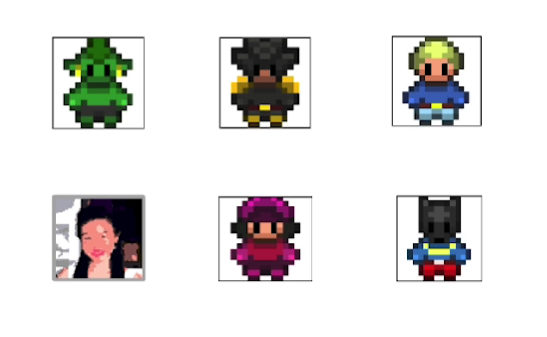
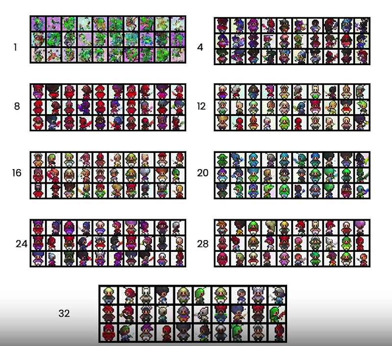
Consider that you have a lot of training data, such as these game character images that you see down here and this is your training data set. You want even more of these game characters that are not represented in your training data set. You can use a neural network that can generate more of these game characters for you, following the diffusion model process.

But the important question that we should answer is how do we make these images useful to the neural network? We want the neural network to learn generally the concept of a game character such as what it is, the hair color of the game character, or that it’s wearing a buckle for its belt. Also the general outlines, like its head and body, and everything in between that.

One way to take your data and be able to emphasize either finer details or general outlines is to add different levels of noise to it. So this is just adding noise to the image, and it’s known as a “noising process”. And this is inspired by physics. You can imagine an ink drop into a glass of water. Initially, you know exactly where the ink drop landed. But over time, you actually see it diffuse into the water until it disappears. And that’s the same idea here, where you start with “Bob the Sprite”, and as you add noise, it will disappear until you have no idea which sprite it actually was.

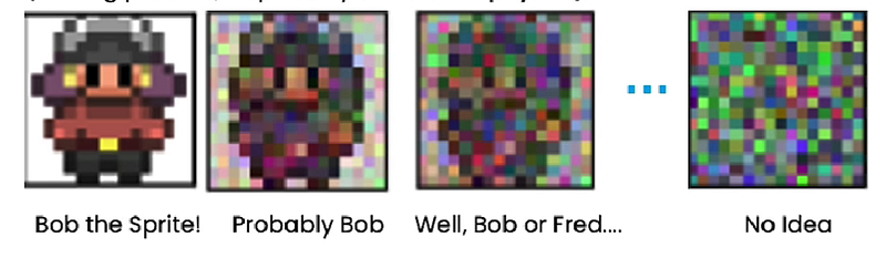
And so what should the neural network really be thinking at each of these levels of noise:

If it’s Bob the Sprite: keep Bob as is
If it’s likely to be Bob: Suggest possible details to be filled in
If it’s just an outline of a sprite: Suggest general details for likely sprites
If it looks like nothing: Suggest an outline of a sprite

Let’s take a look at what that noising process, that process of adding noise progressively looks like over time. And there it goes, an ink drop that’s fully diffused in a glass of water. So now on to training that neural network. So it learns to take different noisy images and turn them back into sprites. That is your goal. And how it does that is it learns to remove the noise you added.

Starting with the “No Idea” level, where it is just pure noise, to starting to give a semblance of maybe there’s a person in there, to look like Fred, and then finally a sprite that looks like Fred.

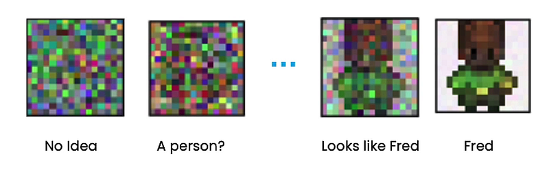
The “No Idea” level of noise is really important because it is normally distributed. Therefore those pixels are sampled from a normal distribution, also known as a “Gaussian distribution” or a “bell-shaped curve”. So when you want to ask the neural network for a new game character, such as Fred here, you can sample noise from that normal distribution, and then you can get a completely new game character by using the neural network to just remove that noise progressively. So now you’ve reached your goal. You can get even more game characters beyond all those that you had trained on.

2. Sampling Technique

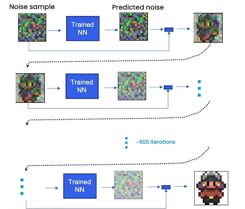
Before we talk about how to train the neural network, let’s talk about sampling or what we do with the neural network after it’s trained at inference time. So what happens is you have that noise sample. You put it through your trained neural network that has understood what a game character looks like and what it does is it predicts noise.

It predicts noise as opposed to the sprite and then we subtract that predicted noise from the noise sample to get something a little bit more sprite-like. Realistically that is just a prediction of noise and it doesn’t fully remove all the noise so you need multiple steps to get high-quality samples. That’s after 500 iterations we’re able to get something that looks very sprite-like.

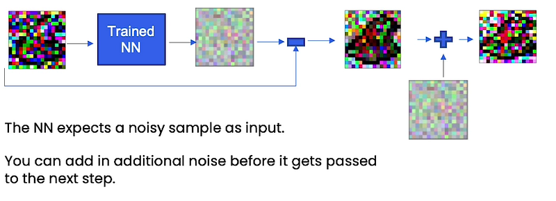
Right now you have your neural network that’s predicting noise from your original noise sample. You subtract it out and then you will get something that looks a little like a game character. However, this neural network expects this noisy sample, this normally distributed noisy sample as input and once you’ve denoised it, it’s no longer distributed in that way. So actually, what you have to do after each step and before each next step is to add in additional noise that’s scaled based on what time step you’re at, to get passed in as the next sample, the next iteration into your trained neural network. Empirically, this helps stabilize the neural network so it doesn’t collapse to something that’s close to the average of the dataset.

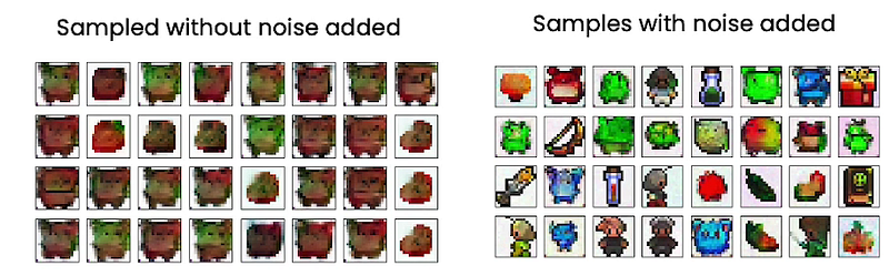
When we don’t add that noise back in, the neural network just produces these average-looking blobs of game characters on the left versus when we go add it back in, it actually is able to produce these beautiful images of game characters shown on the right in the image below.

3. Neural Network

The neural network architecture that we use for diffusion models is a UNet. The most important thing that you need to know about a UNet is that it is taking as input this image, and it’s producing as output something of the same size as that image, but here it is that predicted noise. UNets have been around for a very long time, since 2015, and it was first used for image segmentation. It was first used to take an image and actually segment it into either a pedestrian or a car, so it’s used a lot in self-driving car research.

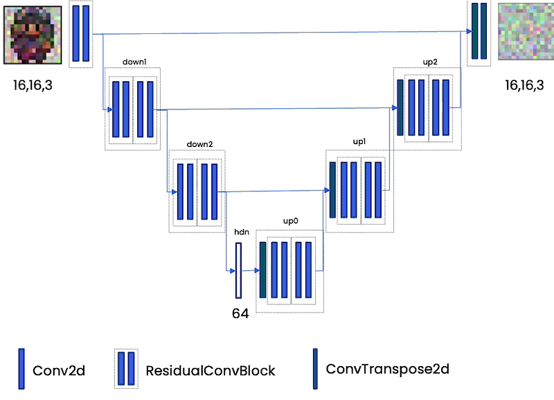
The Unet first embeds information about this input, so it down-samples with a lot of convolutional layers, into an embedding that compresses all that information into a small amount of space. Then it up-samples with the same number of up-sampling blocks into the output back out for its task. In this case that task is to predict the noise that was applied to this image.

Another great capability of UNet is that it can take in additional information. So it compresses the image to understand what’s going on, but it can also take in more information.

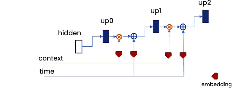
There are two important for these models which are the time and context embedding. Time embedding tells the model the time step and therefore the level of noise we need. All you have to do for this time embedding is embed it into some kind of vector, and you can add it into these up-sampling blocks. The context embedding helps you control what the model generates. For example, a text description, or some kind of factor, like it needs to be a certain color. For that context embedding, you can just multiply it in.

4. Diffusion Model Training

The goal of the neural network is for it to predict noise, and really it learns the distribution of what is noise on the image, but also what is not noise, what is game character likeness.

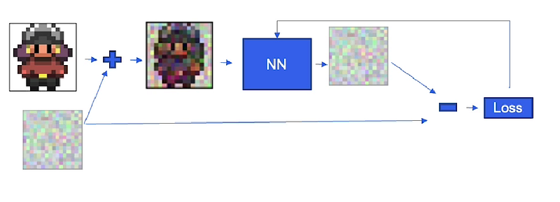
And so how we do that is that we take the game character from our training data, and we actually add noise to it. We add noise to it, and we give it to the neural network, and we ask the neural network to predict that noise. And then we compare the predicted noise against the actual noise that was added to that image, and that’s how we compute the loss. And that backdrops through the neural network, so then the neural network learns to predict that noise better.

So how do you determine what this noise is? You could just go through time and sampling and give it different noise levels. But realistically, in training, we don’t want the neural network to be looking at the same game character all the time. It helps it to be more stable if it looks at different game characters across an epoch, and it’s just more uniform. So actually what we do is we randomly sample what this time step could be. We then get the noise level appropriate to that time step. We add it to this image, and then we have the neural network predict it. We take the next game character image in our training data. We again sample a random time step which could be totally different. Then we add it to this game character image, and again we have the neural network predict the noise that was added. This technique results in a much more stable training scheme.

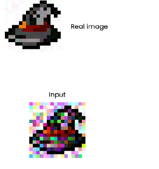
To have a better understanding of what does the training actually look like. Here is a wizard hat of the game character, and here is what a noise input would look like.

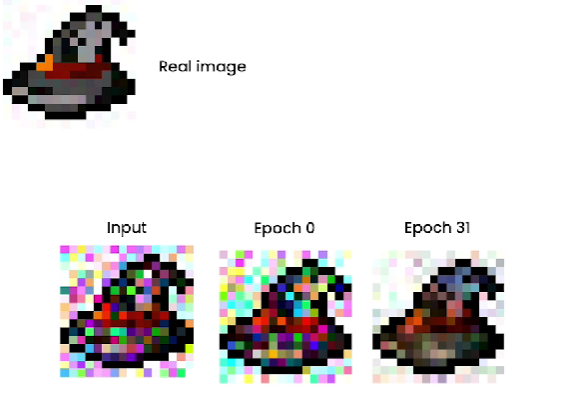
When you first put it into the neural network at epoch 0, the neural network hasn’t really learned what a sprite is yet. So the predicted noise doesn’t quite change what the input looks like, and when it’s subtracted out, it actually just turns out to look about the same. But by the time you get to epoch 31, the neural network has a better understanding of what this sprite looks like. So then it predicts noise, which is then subtracted from this input to produce something that does look like this wizard hat of a game character.

This is just one sample. We can see in the image below multiple different samples, for multiple different game characters, across many epochs, and what that looks like. As you can see in this first epoch, it is quite far from a game character, but by the time you get to epoch 32 here, it looks quite like a little video game character.

Here is a summary of the training of the neural network:

Sample training image
Sample timestep t that determines the level of noise
Sample the noise
Add noise to the image
Input this into the neural network that will predict the noise
Compute loss between predicted and true noise
Backpropagt and make the neural network learn

5. Controlling the Diffusion Model Output

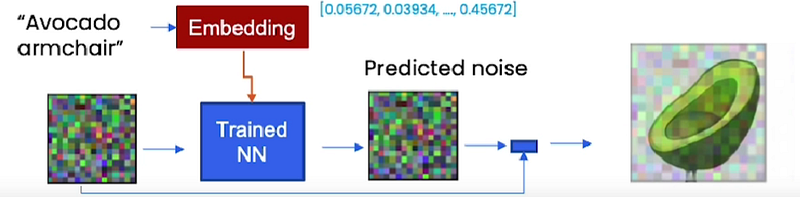
After we have known how the model actually works, let's see how to control the model and what it generates. For many of us, this is the most exciting part because you get to tell the model what you want and it gets to imagine it for you. When it comes to controlling these models, we will use text embeddings. Embeddings are vectors that are able to capture meaning. Here it’s capturing the meaning of sentences through diffusion models. In the example below we can see that it encodes different words, which is this set of numbers in a vector.

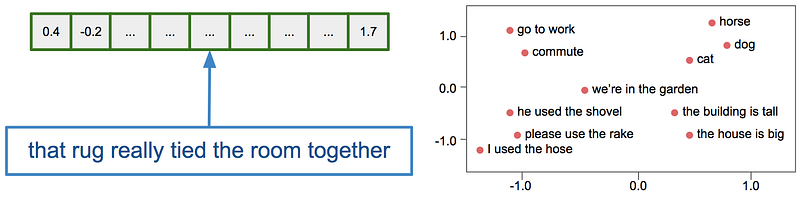
Embeddings are special in that they can capture the semantic meaning, text with similar content will have similar vectors. And one of the kind of magical things about embeddings is you can almost do this vector arithmetic with it.

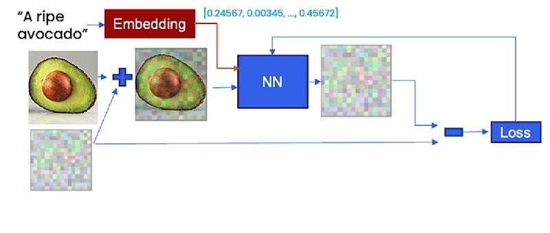
These embeddings provide context to the model during training. For example, here you have an avocado image and you also have a caption for it “A ripe avocado”. You can actually pass that through, get an embedding, and input that into the neural network to then predict the noise that was added to this avocado image and then compute the loss and do the same thing as before.

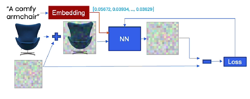
You could do this across a lot of different images with captions. So here is a comfy armchair. You can pass it through an embedding, pass it into the model, and have that be part of training.

Now, the magic of this part is that while you were able to scrape these images of avocados and armchairs off the internet with those captions, you’re able to, at sample time, be able to generate things that the model has never seen before. And that could be an “avocado armchair”. The magic of this is that you can embed the words “avocado armchair” into this embedding that has, a bit of avocado in there, a bit of armchair in there, put that through the neural network, have it predict noise, subtract that noise out and get an “avocado armchair”.

So more broadly context is a vector that can control generation. Context can be, just as we have seen now, the text embeddings of that “avocado armchair” that’s very long. But the context doesn’t have to be that long. Context can also be different categories that are five in length, you know, five different dimensions, such as having a hero or being a non-hero. It could be food items such as an apple, an orange, or a watermelon. It could be spells and weapons like a bow and an arrow or a candle.

6. Speeding Up the Sampling Process

Finally, you’ll learn about a new sampling method that is over 10 times more efficient than DDPM, which is what we’ve been using so far which is called Denoising Diffusion Implicit Models (DDIM). So your goal is that you want more images, and you want them quickly. But sampling so far has been slow because there are many time steps involved, 500 for example and there are even more sometimes to get a good sample, and also each time step is dependent on the previous one as it follows a Markov chain process.

But thankfully, there are many new samplers here to address this problem, since this has been a long-standing problem with diffusion models. It’s that you can train them, and they can create amazing beautiful images that are both diverse and realistic, but it’s so slow to get something out of them.

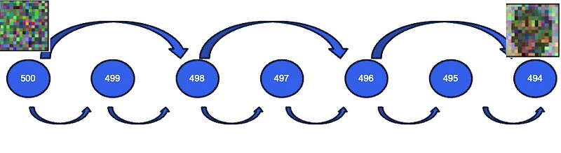
One of these samplers that has been very popular is called DDIM. DDIM is faster because it’s able to skip time steps. So instead of going from time step 500 to 499 to 498, it’s able to skip all these time steps because it breaks the Markov assumption. Markov chains are only used for probabilistic processes. But DDIM actually removes all the randomness from this sampling process and is therefore deterministic. It predicts a rough sketch of the final output, and then it refines it with the denoising process.

So let’s compare DDPM here on the left, which is what we’ve been using so far, and DDIM on the right. You can see that it is much faster with DDIM. You immediately see a book thereafter time step 19 while it goes all the way up to 500 with DDPM.

In this article, we went through the basics of the diffusion model and how it works and what are the main components of it. In the next article, we will implement each of these components to have a better understanding of each of them.

References

How Diffusion Models Work