How I Maximize Market Returns to a Win Rate of 65% with Volatility-Bollinger Bands 🤩

Implementing and backtesting techniques can be a useful tool for traders to evaluate the viability of their trading ideas in the realm of stock trading. The Volatility using the Bollinger Bands strategy is one of them. We will go into detail about this strategy in this article and show you how to put it to the test using Python.

Let’s quickly review the data preparation procedure before moving on to the strategy itself. In a previous article titled “Backtesting Stock Trading Strategies Using Python (Data Preparation),” we discussed how to get online OIH stock data and create files with data in several timeframes, including 1-minute, 5-minute, 15-minute, 1-hour, and 1-day intervals.

These files will serve as the input for testing our Volatility with Bollinger Bands strategy.

We also prepared an environment to test any strategy generating buy and sell signals which we are going to use to generate this backtest.

Before I continue sharing all the information, if you enjoy reading my articles, please hit the follow button — Diego Degese

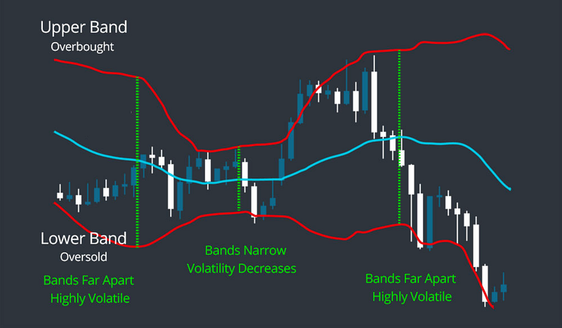
Understanding the Volatility with Bollinger Bands Strategy

The heart of our approach lies in the get_signals method. This method takes a DataFrame as input and calculates buy and sell signals based on the selected strategy. Let's examine the code step by step:

import numpy as np
import pandas as pd
import pandas_ta as ta

# ...

def get_signals(df):
    pd.options.mode.chained_assignment = None
    
    df.ta.bbands(close=df['close'], length=20, append=True)    
    df = df.dropna()
    
    df['high_limit'] = df['BBU_20_2.0'] + (df['BBU_20_2.0'] - df['BBL_20_2.0']) / 2
    df['low_limit'] = df['BBL_20_2.0'] - (df['BBU_20_2.0'] - df['BBL_20_2.0']) / 2
    df['close_percentage'] = np.clip((df['close'] - df['low_limit']) / (df['high_limit'] - df['low_limit']), 0, 1)
    df['volatility'] = df['BBU_20_2.0'] / df['BBL_20_2.0'] - 1
    min_volatility = df['volatility'].mean() - df['volatility'].std()
    
    df['signal'] = np.where((df['volatility'] > min_volatility) & (df['close_percentage'] < 0.25), 1, 0)
    df['signal'] = np.where((df['close_percentage'] > 0.75), -1, df['signal'])
    
    return df['signal']

Let’s break down the code and understand each step:

First, we import the necessary libraries: numpy as np, pandas as pd, and pandas_ta as ta.

Then we define the get_signals method that takes the DataFrame df as input.

We use the ta.bbands function from the pandas_ta library to calculate the Bollinger Bands. We pass the closing price (df['close']) and set the length parameter to 20 (which is the most used value). The append=True parameter ensures that the Bollinger Bands columns are appended to the DataFrame.

Next, we calculate the high and low limits of the working range (the upper Bollinger Band is represented by 0.75 or 75% of the range, and the lower Bollinger Band is represented by 0.25 or 25% of the range, giving space to the price when it goes over or under the bands). The high limit is obtained by adding half the width of the Bollinger Bands to the upper band value (represented by 1 or 100% of the range), while the low limit is obtained by subtracting half the width of the Bollinger Bands from the lower band value (represented by 0 or 0% of the range).

We calculate the close percentage, which represents the position of the closing price relative to the working range. It is calculated as the clipped value of the difference between the closing price and the low limit divided by the range between the high and low limits.

The volatility is computed as the ratio between the upper and lower Bollinger Bands minus 1.

We determine the minimum volatility required to open a position by subtracting the standard deviation of the volatility from its mean.

Buy Signals

Based on our strategy, we assign a buy signal (1) when the volatility is greater than the minimum volatility required and the close percentage is less than 0.25.

Sell Signals

Similarly, we assign a sell signal (-1) when the close percentage exceeds 0.75.

Backtesting and Analyzing the Results

To evaluate the performance of the volatility with Bollinger Bands strategy, the following code snippet provides the show_strategy_result method. This method simulates a long position strategy and calculates the profit/loss, number of wins, losses, and win rate.

def show_strategy_result(timeframe, df):
    waiting_for_close = False
    open_price = 0

    profit = 0.0
    wins = 0
    losses = 0
    
    for i in range(len(df)):
        signal = df.iloc[i]['signal']
        
        if signal == 1 and not waiting_for_close:
            waiting_for_close = True
            open_price = df.iloc[i]['close']
        elif signal == -1 and waiting_for_close:
            waiting_for_close = False
            close_price = df.iloc[i]['close']

            profit += close_price - open_price
            wins += 1 if (close_price - open_price) > 0 else 0
            losses += 1 if (close_price - open_price) < 0 else 0

    print(f' Result for timeframe {timeframe} '.center(60, '*'))
    print(f'* Profit/Loss: {profit:.2f}')
    print(f"* Wins: {wins} - Losses: {losses}")
    print(f"* Win Rate: {100 * (wins/(wins + losses)):6.2f}%")

If you run this code with the data provided in the first article, you should see something similar to this.

***************** Result for timeframe 5T ******************
* Profit/Loss: 2403.68
* Wins: 3379 - Losses: 1851
* Win Rate:  64.61%
***************** Result for timeframe 15T *****************
* Profit/Loss: 2220.58
* Wins: 1369 - Losses: 726
* Win Rate:  65.35%
***************** Result for timeframe 1H ******************
* Profit/Loss: 251.15
* Wins: 417 - Losses: 203
* Win Rate:  67.26%
***************** Result for timeframe 1D ******************
* Profit/Loss: -122.69
* Wins: 43 - Losses: 19
* Win Rate:  69.35%

Conclusion

In this article, we explored the Volatility with Bollinger Bands strategy for stock trading and demonstrated how to test it using Python. By understanding the code and following the step-by-step explanation, you can now apply this strategy to analyze and evaluate stock trading opportunities across different timeframes. Remember to adjust and optimize the strategy parameters based on your specific requirements and market conditions to enhance its effectiveness.

Bonus

Trying to push the boundaries and improve the performance of the Volatility with Bollinger Bands strategy, I created another article that uses a Genetic Algorithm to find the best parameters to generate the buy and sell signals achieving a win rate of 75% and also improving the profit/loss.

If you enjoy my work, please support me on Medium by becoming a member through my referral link, and consider giving it a clap as a small gesture of motivation. Thank you!

Download the full source code and the colab notebook of this article from here

Twitter / X: https://twitter.com/diegodegese LinkedIn: https://www.linkedin.com/in/ddegese Github: https://github.com/crapher

Disclaimer: Investing in the stock market involves risk and may not be suitable for all investors. The information provided in this article is for educational purposes only and should not be construed as investment advice or a recommendation to buy or sell any particular security. Always do your own research and consult with a licensed financial advisor before making any investment decisions. Past performance is not indicative of future results.