Unlocking Insights from Multivariate Data with the Temporal Fusion Transformer

Probabilistic Forecast of a Multivariate Time Series using the Temporal Fusion Transformer & PyTorch Lightning

Time series forecasting is the science/art of developing models that predict future values based on historical information. It’s used across many industries for tasks ranging from stock market price prediction, sales, and revenue forecasting, and prediction of inventory or resource management requirements to engineering signal analysis.

Deep neural networks (DNNs) have increasingly been used to perform multi-horizon time series forecasting as they’ve been shown to outperform classical time series models. In this article, I will walk through the process of using deep learning to perform a probabilistic forecast of a multivariate time series. The Google Temporal Fusion Transformer (TFT) will serve as our neural network architecture, and PyTorch Lightning (now just called Lightning) as our computational framework. I developed the Jupyter notebook in Google Colab because they provide access to much nicer GPUs than I’ve got at home :)

The topics covered in this article include:

• Data exploration and analysis of our covariate dataset
• How to prepare the data for use by the TFT model
• How to create, train and evaluate the TFT model
• How to generate and review model predictions from both the validation data and out-of-sample predictions

Model Architecture

The Google research team introduced the Temporal Fusion Transformer architecture in late 2019. The standard transformer architecture (i.e., GPT-3, ChatGPT) utilizes one too many attention heads for identifying long-term patterns in a time series. In addition to the transformer attention heads, the TFT includes LSTM (Long Short Term Memory) cells for managing shorter duration patterns and for providing context with surrounding values, as well as GRNs (Gated Residual Networks) that act as gates for filtering out unimportant information.

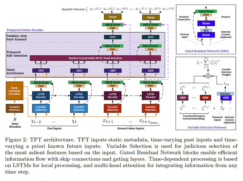
A great overview of the Temporal Fusion Transformer is provided in the following blog: Google Research — Interpretable Deep Learning for Time Series Forecasting.

Data Exploration & Analysis

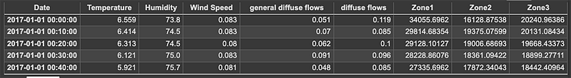
The dataset used for this example is electric power consumption data from the city of Tetouan. Tetouan is a city just north of Morocco which occupies an area of around 10,375 km² and has a population of about 550,374. The energy distribution network is powered by three-zone stations (Quads, Smir and Boussafou). The following energy and weather-related data were collected in 10-minute intervals over the course of a year:

• Power consumption per zone
• General diffuse flows
• Diffuse flows
• Temperature
• Humidity
• Wind Speed

The goal of this analysis is to create a neural network model that can accurately predict future power consumption load per distribution zone.

Loading the data into a Pandas dataframe yields:

To make our predictions more useful, I aggregate the data into hourly samples and then check for any missing data.

data_hr = df.resample('1h').mean()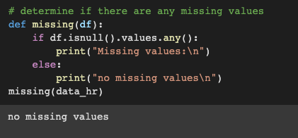

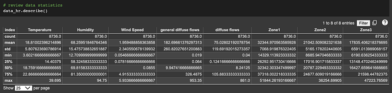
Then review our dataset statistics:

Data Wrangling

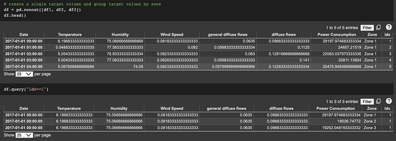
The goal of our analysis is to forecast the power consumption per zone, so our target variable is ‘power consumption’. For input into the TFT model, we need to rearrange our dataframe so that the target variables are in a single column. The approach I took (and am sure pretty sure there is a more elegant approach) was to split our base dataframe into individual dataframes per zone, add a zone identifier and time index to each respective component dataframe and then concatenate them into a new dataframe with a single ‘power consumption’ column.

Feature Engineering

In order to assist the TFT model in capturing energy use patterns across different times of the day, days of the week, or weather changes per month, date/time-based features are added to our dataframe.

# create time-based features to help our model capture seasonality aspects
date = df.index
df['Hour'] = date.hour
df['WeekDay'] = date.dayofweek
df['Month'] = date.month
df.head(10)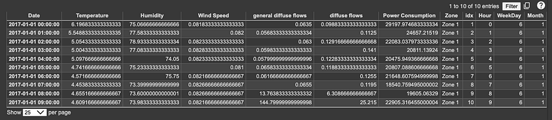

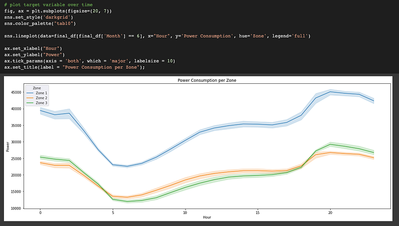
Let’s take a look at the power consumption per zone on a given day.

Data Analysis

Next, let’s review any correlations between power consumption and our various covariates. The analysis indicates that there is little to no correlation between power consumption and the diffuse flows, WeekDay, and Month covariates.

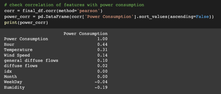
# create correlation matrix
corr_idx = final_df.corr().sort_values("Power Consumption", ascending=False).index
corr_sorted = final_df.loc[:, corr_idx]  

plt.figure(figsize = (12,12))
sns.set(font_scale=0.75)
ax = sns.heatmap(corr_sorted.corr().round(3), annot=True, square=True, 
      linewidths=.75, cmap="coolwarm", fmt = ".2f", annot_kws = {"size": 11})
ax.xaxis.tick_bottom()
plt.title("Correlation Matrix")
plt.show()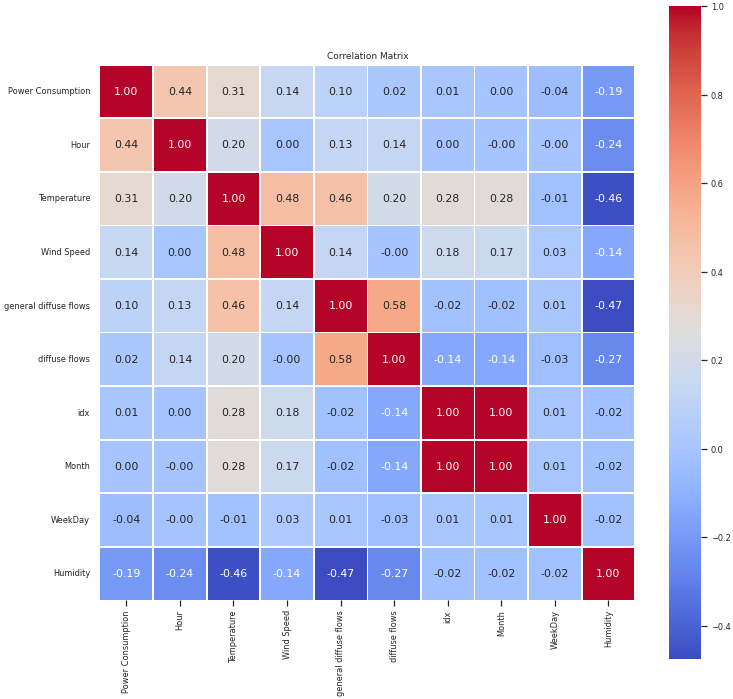

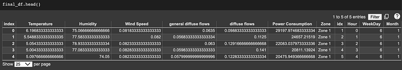
A view of our final dataframe for input into the TFT model.

Create & Train the TFT Model

So far, we’ve just been using Python and Pandas to load, explore, and prep our data for input into the neural network model. Moving forward, we will leverage various deep learning libraries. You can install the PyTorch Lightning and PyTorch Forecasting libraries using the following command:

pip install torch pytorch-lightning pytorch_forecasting

Import the deep learning libraries.

# import deep learning libraries
import pytorch_lightning as pl
from pytorch_lightning.callbacks import EarlyStopping, LearningRateMonitor
from pytorch_lightning.loggers import TensorBoardLogger
import torch

from pytorch_forecasting import TemporalFusionTransformer, TimeSeriesDataSet
from pytorch_forecasting.data import GroupNormalizer
from pytorch_forecasting.metrics import QuantileLoss
from torchmetrics import MeanAbsolutePercentageError
from pytorch_forecasting.models.temporal_fusion_transformer.tuning 
                                    import optimize_hyperparameters

import tensorflow as tf 
import tensorboard as tb 
tf.io.gfile = tb.compat.tensorflow_stub.io.gfile

import warnings
warnings.filterwarnings('ignore', category=FutureWarning)

You will also need to install the TensorFlow deep learning library in order to use tensorboard to review the execution outputs. You will need to search how to install it on your respective hardware because the installation process varies from platform to platform.

Before creating our deep learning model, I want to highlight a few attributes that make the Temporal Fusion Transformer unique.

• Unlike most neural network models, the TFT can process and be trained on multiple univariate or multivariate time series at once — here, power consumption for 3 separate zones
• The TFT can output multi-step predictions of our target variable, including probabilistic prediction intervals
• The TFT model supports multiple feature input streams, including time-varying knew, time-varying unknown, time-invariant real, and time-invariant categorical features
• Unlike many time series models, the TFT does not require a stationary time series for training
• The TFT model provides insight and understanding into the covariate feature importance and attention values used for time series predictions

The final two steps to prepare our data for input into the TFT model are:

• Instantiate PyTorch Forecasting TimeSeriesDataSet objects for our training and test datasets
• Create our data loaders for iteratively passing data to the TFT model

The TimeSeriesDataSet class enables us to specify how our input features should be utilized by the model, enables feature normalization and makes creating the data loaders super easy. It is also the only input format that the TFT model will accept.

TimeSeriesDataSet & Data Loaders

The frequency of our data is hourly. We’ll use a ‘look back window’ of one week’s worth of data (24 hrs. x 7 days) for predicting/forecasting the power consumption for the next 24 hours.

# create Time Series Dataset Objects
lookback = 24 * 7
prediction_length = 24

train_split = final_df["idx"].max() - prediction_length

training = TimeSeriesDataSet(final_df[lambda x: x.idx <= train_split], time_idx="idx", target="Power Consumption", group_ids=["Zone"], 
                             min_encoder_length=lookback // 2, max_encoder_length=lookback, min_prediction_length=1, 
                             max_prediction_length=prediction_length, static_categoricals=["Zone"], time_varying_known_reals=["idx", "Hour"],
                             time_varying_unknown_reals=["Temperature", "Humidity", "Wind Speed", "general diffuse flows", "Power Consumption"], 
                             target_normalizer=GroupNormalizer(groups=["Zone"], transformation="softplus"), add_relative_time_idx=True, 
                             add_target_scales=True, add_encoder_length=True)

validation = TimeSeriesDataSet.from_dataset(training, final_df, predict=True, stop_randomization=True)

A few notes:

• The target variable is our Power Consumption, grouped by Zone
• The Zone is also classified as a categorical input feature
• The time-varying known real features are idx and Hour; where idx is our marching forward time index
• The time-varying unknown real features are: Temperature, Humidity, Wind Speed, general diffuse flows, and Power Consumption
• I did not include the diffuse flows, Weekday or Month features because of their low correlation to Power Consumption
• Note the use of the GroupNormalizer to normalize the input features

Now creating the data loaders is a piece of cake:

# create our data loaders
batch_size = 32
train_dataloader = training.to_dataloader(train=True, 
                   batch_size=batch_size, num_workers=2)
val_dataloader = validation.to_dataloader(train=False, 
                    batch_size=batch_size, num_workers=2)

Create & Train the TFT Model

To create the TFT neural network model, you instantiate an instance from the PyTorch Forecasting TemporalFusionTransformer class.

# create our TFT model
tft = TemporalFusionTransformer.from_dataset(
training, learning_rate=0.001, hidden_size=128, attention_head_size=4, 
dropout=0.1, hidden_continuous_size=128, output_size=7, loss=QuantileLoss(),
reduce_on_plateau_patience=4)

Note the assigned loss function - QuantileLoss. Using the quantile loss function, the model will output probabilistic, rather than a point, predictions. The quantile loss function was first proposed in the following paper Wen et al and was later implemented by Amazon engineers in their GluonTS model.

We’ll use the PyTorch Lightning Trainer to manage the model training process. It assists with a number of execution processes, such as automatically capturing training checkpoints and key model performance metrics. This is also where we define our acceleration options and callback methods. The trainer is defined by invoking the PyTorch Lightning Trainer class.

# define our Pytorch Lightning Trainer & Callbacks
early_stop_callback = EarlyStopping(monitor="val_loss", min_delta=1e-4, 
                      patience=5, verbose=True, mode="min")
lr_logger = LearningRateMonitor()
logger = TensorBoardLogger("/drive/My Drive/logs/lightning_logs2")  

epochs = 50
trainer = pl.Trainer(max_epochs=epochs, accelerator='gpu', devices=1, 
          enable_model_summary=True, gradient_clip_val=0.1, 
          callbacks=[lr_logger, early_stop_callback], logger=logger)

Model training is initiated by the trainer.fit command.

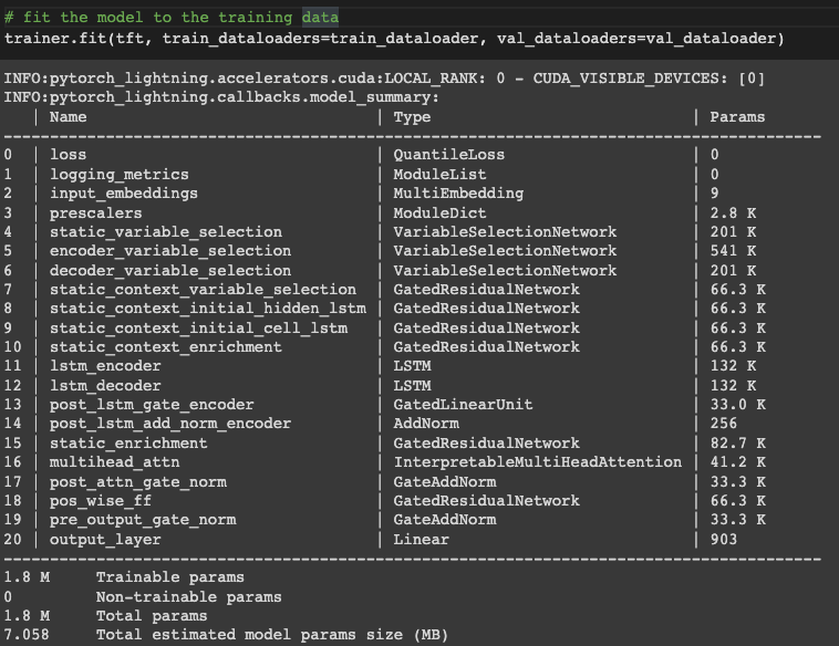
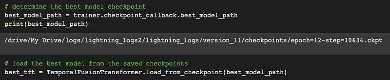
Due to the use of the early stopping callback, the training process completes after 12 epochs. The inference model is created by loading the best training checkpoint into our TFT model.

Model Results & Predictions

Tensorboard is used to review the model training metrics. Tensorboard can be executed within a Jupyter notebook by invoking the below commands.

# Start tensorboard
%load_ext tensorboard
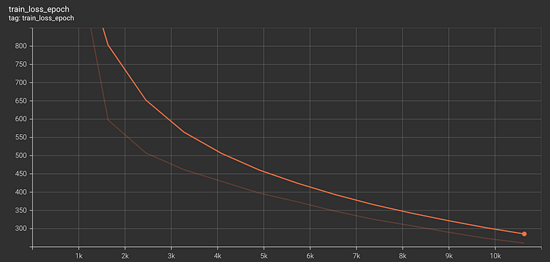
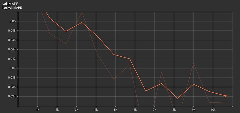
%tensorboard --logdir "/drive/My Drive/logs/lightning_logs2/lightning_logs/version_11"

Model Training Metrics

The model was performed with a validation MAPE (Mean Absolute Percentage Error) of 0.034.

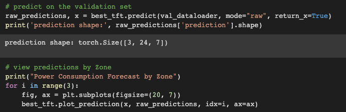
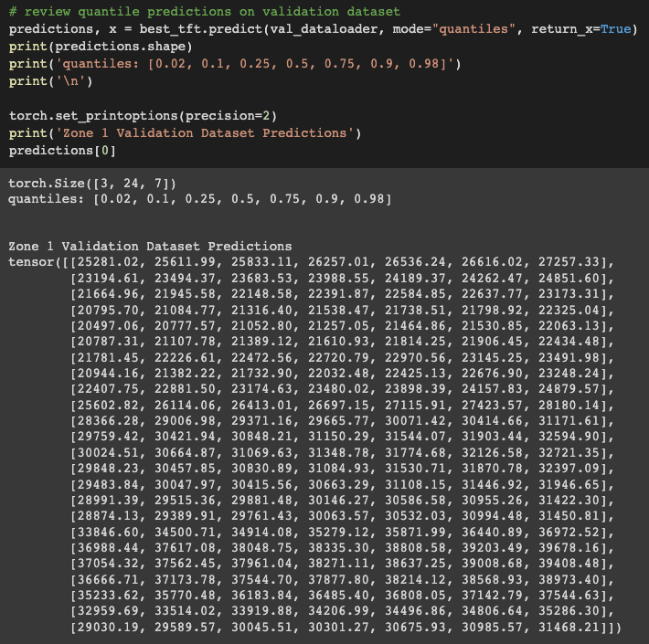
Test Predictions

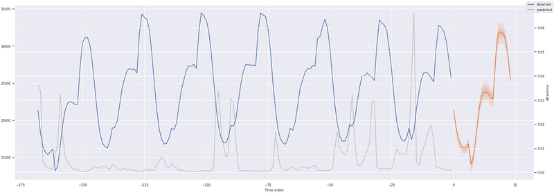
Next, we review the probabilistic forecast predictions for each zone in our validation data. Note the shape of the prediction tensor — 3 zones x 24 hours x 7 quantiles.

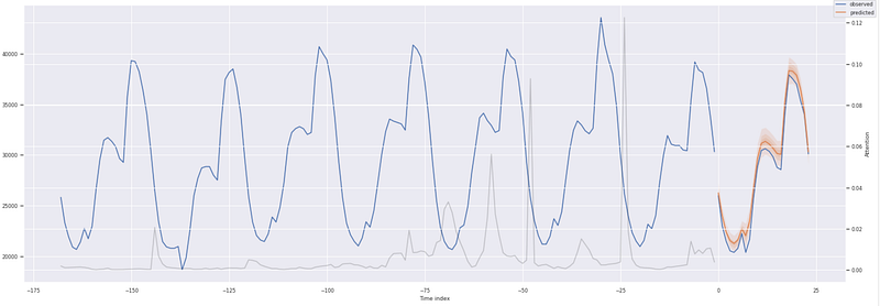
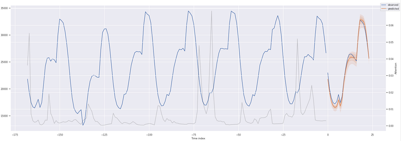
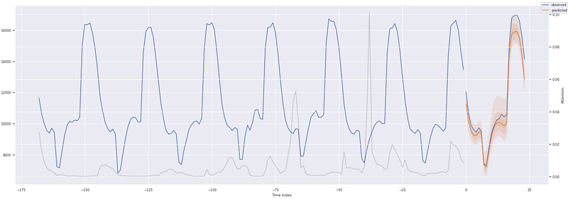
Items to note about the prediction plots.

• The dark orange line is the 50% or median quantile value prediction
• The lighter shades of orange are the various quantile prediction bands around the median and denote the range of the predictions
• The gray line shows the amount of attention the model pays to different points in the time when making the predictions

For the initial run, the TFT model did a great job of capturing the behavior and trends of the power consumption usage across all 3 zones with a validation MAPE of 0.034. Model performance could be improved further by performing hyperparameter optimization, including varying the look-back window. PyTorch Forecasting has an ‘optimize_hyperparameters’ library that can be used to assess various hyperparameter permutations.

We can directly compare the predictions for a given zone to the validation data. The quantile loss function provides a range of probabilistic prediction values. Note the prediction tensor shape for a single zone — 24 hrs. x 7 quantiles.

• Zone 1 50% quantile prediction — 26,257
• Zone 1 validation data power consumption — 25,985

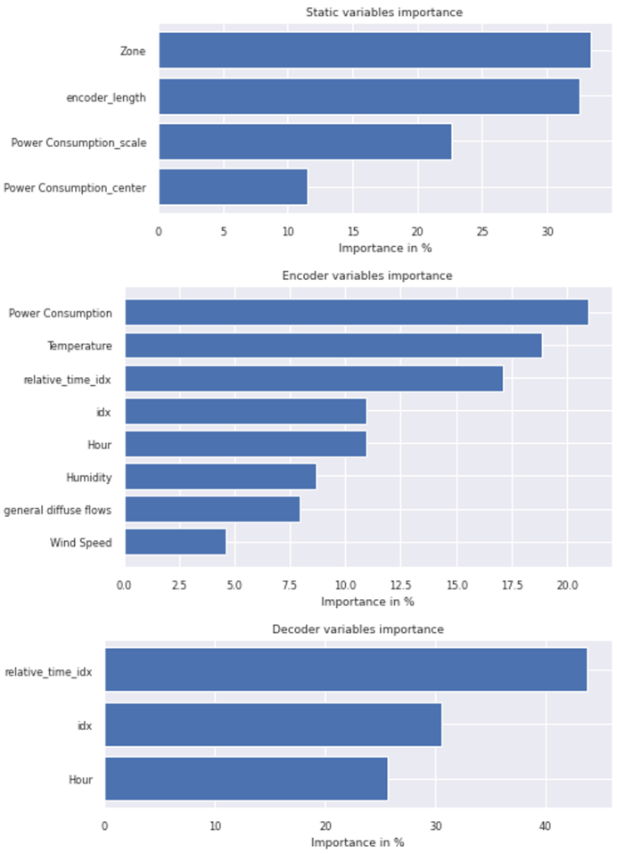
Feature Level Interpretability

One of the great attributes of the TFT model is that it enables an easy understanding of the temporal attention and feature prioritization the model used to generate its prediction forecast.

# feature level interpretability
raw_predictions, x = best_tft.predict(val_dataloader, mode="raw", 
                     return_x=True)
interpretation = best_tft.interpret_output(raw_predictions, reduction="sum")
best_tft.plot_interpretation(interpretation);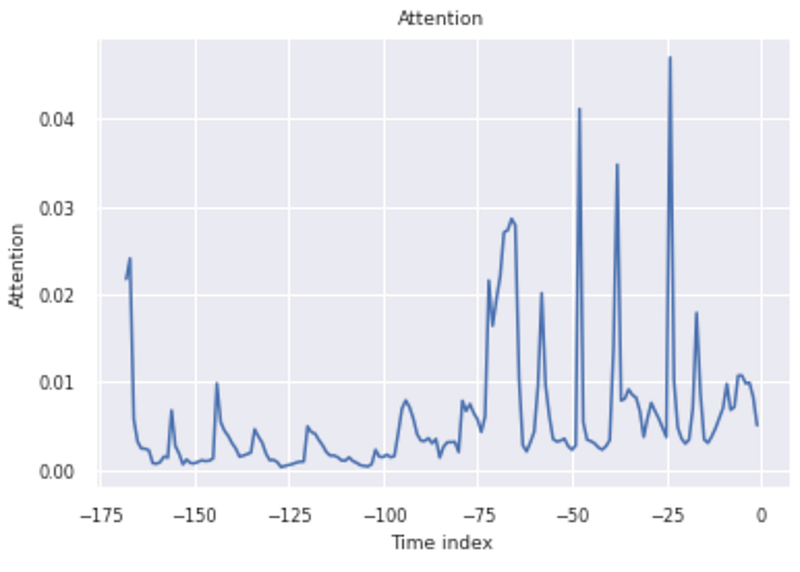

Out-of-Sample Predictions

In order to perform out-of-sample predictions (i.e., predictions beyond the validation data), we need to create an input dataframe that includes the following:

• The necessary historical data for the encoder portion of the model. This would be one look-back window’s worth of data. In our case, this would be 24 hours x 7 days for each of the three zones.
• For the decoder portion of the model, we need to provide future known covariates for the duration of our prediction period (24 hours) for each prediction time series (zone).

The approach is to create the encoder and decoder data as separate respective dataframes and then concatenate them together. Creating the encoder dataframe is easy.

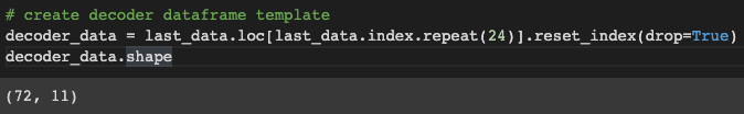
# create decoder data
encoder_data = final_df[lambda x: x.idx > x.idx.max() - lookback]

Creating the decoder data is a bit more involved. We repeat the last set of hourly measurements 24 times and then fix/clean up the covariate column data. First, we figure out where we left off from the validation data.

# our last validation data points
last_data = final_df[lambda x: x.idx == x.idx.max()]
last_data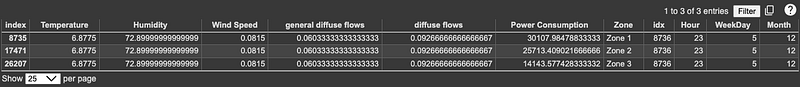

Now we repeat the last set of rows 24 times. Note the length of 72, 24 hrs. x 3 zones.

So our decoder dataframe now looks as follows:

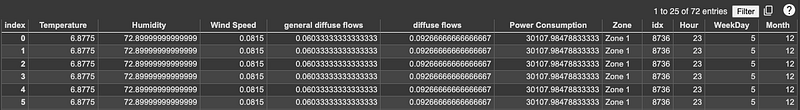
In lieu of better information, we leave the weather and energy data as it was at the end of the day on 12/30/17. Since our out-of-sample prediction is for the 24 hours that make up 12/31/17, the Month covariate data is fine. The WeekDay update is easy, we just bump it from a 5 to a 6. Then for each of the three zones:

• Increment the time index (idx) forward by 24 from where the validation data left off at 8736
• Update the Hour data to run from 0–23 for our prediction period of 24 hours

Finally, we concatenate the encoder and decoder dataframes together to form our input inference dataset.

# now create our combined prediction dataset dataframe
new_pred_data = pd.concat([encoder_data, decoder_data], ignore_index=True)
new_pred_data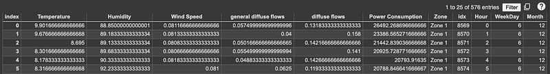

Now we make out-of-sample predictions from our inference dataset.

# make & plot out of sample predictions
inf_raw_predictions, inf_x = best_tft.predict(new_pred_data, 
                             mode="raw", return_x=True)

for i in range(3):    
    fig, ax = plt.subplots(figsize=(20, 7))
    best_tft.plot_prediction(inf_x, inf_raw_predictions, idx=i, 
                             show_future_observed=False, ax=ax)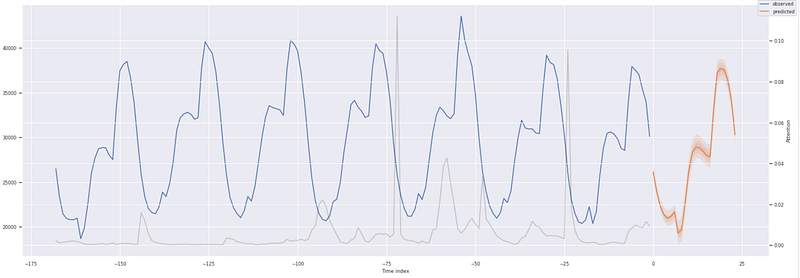

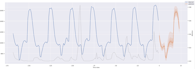
Concluding Remarks

In the Google technical paper, the authors compared the TFT model performance against numerous current state neural network models and classical methods. The TFT out performed them all. As shown above, the Temporal Fusion Transformer provides state-of-the-art results in a manner that enables understanding and interpretability of the results.

Unlike most time series prediction models, the TFT model easily handles multivariate heterogeneous features and enables the prediction of multiple time series within a single training run. When paired with the quantile loss function, it provides a range of predictions as opposed to only point estimates which can greatly improve prediction confidence and help facilitate actionable decision-making.

Thank you so much for reading this far; I hope you enjoyed the article. You can find the Jupyter notebook for this article on my GitHub site.

Cheers :)

Reference Notes

• Unless denoted otherwise, all images were created by the author from the Jupiter notebook code.