Understanding The Kernel Trick In Machine Learning — Part 1

In this series of articles, we want to understand what is meant by the ‘kernel trick’. We want to both understand the idea behind it and how it can be used in practice. This is the first part of the series, which means we will need to lay down a base before we can get truly started. Therefore, in this article, we will look at a, hopefully, well-known friend: Linear Classification. In this article, we will only consider binary classification. In later articles, we will talk more about Support Vector Machines.

The Intuition Behind Linear Classification

So, what exactly is the idea behind binary Linear Classification? Well, imagine that we have two classes of data: red and blue. We can say that we have:

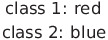
Now, the idea behind linear classification is that we will be able to separate, and thereby classify, our data using a straight line. Let us take an illustrative example:

Here, we can call the straight line our decision boundary. This simply means that it is the boundary between our two classes — so if you are on one side, it belongs to class red, and if you are on the other, it belongs to class blue.

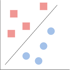
It can, of course, happen that it is not possible for our data to be separated by using a straight line. Imagine it had instead looked like so:

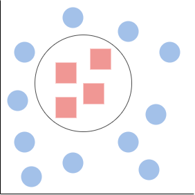
In this case, the circle is our decision boundary. It could also simply have been that it had looked like so:

In both cases, we would not be able to use a straight line to separate them completely from each other. Luckily, we do not need to break our heads on how to handle these cases — yet.

The Math Behind Linear Classification

We have now understood the intuition behind the linear classification. We now need to understand how exactly we define and find this decision boundary.

First of all, we remember that we need to divide our data into one of two classes. In other words, each piece of data is tied to a label, y. Now, instead of defining them to be either ‘red’ or ‘blue’, we define them to be either ‘-1’ or ‘1’. We can write this like so:

Now we need to understand how to find the decision boundary, such that all our data pieces will be defined as one of these classes. Unfortunately for us, this is a rather long explanation. We need to talk about a so-called neuron — yes, the name is inspired by the same neurons that we have in our brains. Now, if you know nothing about neurons, both in a neuroscience or machine learning setting, then don’t worry about it. All we need to know will be explained now.

Let us first take a look at how our neuron, the machine learning one, looks. It can be seen here:

Now, let us try to understand what exactly is going on here. However, let us first cover one important thing we need to remember: the inputs define how many dimensions there are in our data. It does not tell us how many samples there are in our data. In other words, if we have 2 inputs it means that we have 2-dimensional data but we might have much more than 2 samples. This also means that if we have 2-dimensional data, then we only need to find 2 weights. We can then define the following parts:

• Inputs: Defined in a vector (or matrix, depending on dimensions) denoted by ‘x’.
• Weights: Defined in a vector (or matrix, depending on dimensions) denoted by ‘w’.
• Bias: Simply denoted by ‘b’, which is added when we have summed our inputs and weights together.
• Activation Function: When we have summed our inputs and weights together and added the bias, then we need to run our result through an activation function. This is simply a function, which will process the result and turn it into one of our desired outputs.
• Output: Simply denoted by ‘y’, which is supposed to be one of our labels above.

So, let us look closer at the sum. It can be defined as a function, and mathematically, it would look like so:

We could also write it with linear algebra — which would look like so:

Here it is important to remember that ‘w’ is the matrix consisting of all the weights while ‘x’ is the matrix of inputs. Your question might then be: “Okay, but how exactly does this give us a decision boundary? So far, I have not noticed any connection between these neurons and our straight line.”. Well, we need to set it equal to zero such that we have:

This creates a hyperplane that divides the input space into two half-spaces corresponding to the two classes. Hence, we have now found a method to calculate our decision boundary. It is simply all the points that lie on the line defined above.

Now, are we done? No! We still have to find a way to divide our data into one of the two classes. We can do this by creating an activation function defined by:

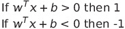
Hence, if a data piece lies above the boundary, then we will classify it as class ‘1’. On the other hand, if it lies beneath the decision boundary then we will classify it as class ‘-1’.

An Example Of The Decision Boundary

We have now understood how the decision boundary is found theoretically. However, let us try to take an example to make it clearer for us how it’s done in practice.

Now, we know that we need both the bias and the weights to find the boundary. Are we always that lucky that we know from the start what these values are supposed to be, such that they correctly classify all our data? It would be nice, but that is not the case at all. However, in this article, we will not show how these values are found. It will instead be saved for a future article since it is a much longer ordeal, especially since we will show how to find the optimal hyperplane (here, the hyperplane is simply our boundary in higher dimensions). Instead, we will take an example where we already know these values and see how the boundary is calculated.

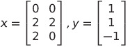
Imagine that we have the following data and their corresponding labels:

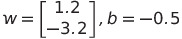
We can then say that we have found the weight and bias to be equal to:

We then find the decision boundary by using the following formula from above:

This gives us:

This means that our decision boundary is equal to:

If we look at it visually, we can see that we have:

We can then see that the activation function:

Makes it such that the points (0,0) and (2,2) are assigned the label ‘1’, while (2,0) is assigned the label ‘-1’.

Conclusion

We have now laid down a basic knowledge of binary linear classification. We have understood the intuition behind it, while also seeing how we can calculate the boundary when we have all the values. In later articles, we will look at how these values can be calculated while also trying to find the ‘optimal hyperplane’. However, in the next article, we will start talking about kernels and the idea behind the kernel trick.

References

• Igel, C. (2021). Support Vector Machines — Basic Concepts. In Machine Learning: Kernel-based Methods Lecture Notes(Version 0.4.3). Department of Computer Science University of Copenhagen.
• Abu Mostafa, Y. S. Magdon-Ismail, M. Lin, H.T. (2012). Support Vector Machines. In LEARNING FROM DATA — A Short Course. AMLbooks.com.