
Fundamentals
Understanding the Covariance Matrix
All you need to know about variance, standard deviation, correlation, and covariance

Linear algebra is one of the fundamentals of machine learning and is considered the ‘mathematics of data’. While I personally enjoy many aspects of linear algebra, some concepts are not easy to grasp at first. I often struggled to imagine the real-world application or the actual benefit of some concepts.
The covariance matrix, however, tells a completely different story.
The concepts of covariance and correlation bring some aspects of linear algebra to life. Algorithms, like PCA for example, depend heavily on the computation of the covariance matrix, which plays a vital role in obtaining the principal components.
In the following sections, we are going to learn about the covariance matrix, how to calculate and interpret it. But first of all, we need to learn about the related concepts, the basics, allowing us to gain a deeper understanding.
What is correlation and what does it tell us?
Correlation analysis aims to identify commonalities between variables.
Let’s imagine, we measure the variables ‘height’ and ‘weight’ from a random group of people. In general, we would expect the taller people to weigh more than the shorter people. A scatterplot of such a relation could look like this:
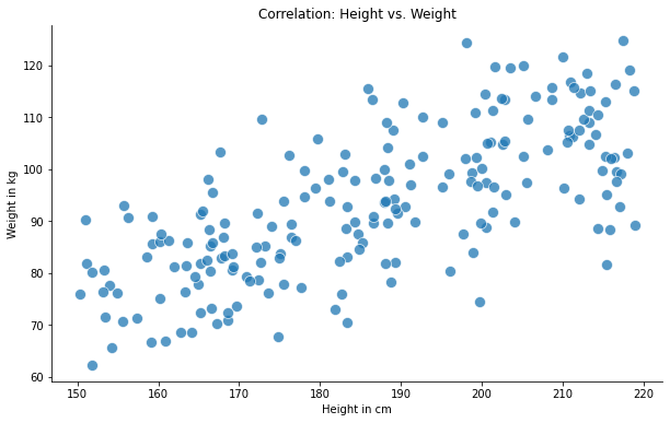
By looking at the plot above, we can clearly tell that both variables are related. Correlation, or more specifically the correlation coefficient, provides us with a statistical measure to quantify that relation.
The coefficient ranges from minus one to positive one and can be interpreted as the following:
- Positive correlation — tells us that both variables move in the same direction e.g. both values are increasing simultaneously.
- Negative correlation — describes inversely correlated variables. Meaning, if one variable is increasing the other is decreasing or vice-versa.
- A correlation coefficient of zero shows that there is no relationship at all.
Note: The correlation coefficient is limited to linearity and therefore won’t quantify any non-linear relations. To measure non-linear relationships one can use other approaches such as mutual information or transforming the variable.
So why do we even care about correlation?
It turns out that the correlation coefficient and the covariance are basically the same concepts and are therefore closely related. The correlation coefficient is simply the normalized version of the covariance bound to the range [-1,1].
Both concepts rely on the same foundation: the variance and the standard deviation.
Introducing variance and standard deviation
Variance as a measure of dispersion, tells us how different or how spread out our data values are.
We can compute the variance by taking the average of the squared difference between each data value and the mean, which is, loosely speaking, just the distance of each data point to the center.
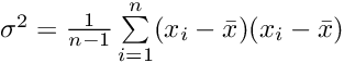
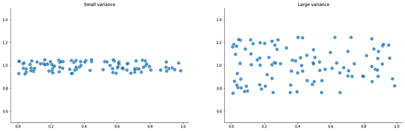
By looking at the equation, we can already tell, that when all data values are close to the mean the variance will be small. If the data points are far away from the center, the variance will be large.
Let’s take a look at two examples to make things a bit more tangible.
Once we know the variance, we also know the standard deviation. It is simply the square root of the variance.

Now that we know the underlying concepts, we can tie things together in the next section.
Covariance and the covariance matrix
Assume, we have a dataset with two features and we want to describe the different relations within the data. The concept of covariance provides us with the tools to do so, allowing us to measure the variance between two variables.
We can calculate the covariance by slightly modifying the equation from before, basically computing the variance of two variables with each other.
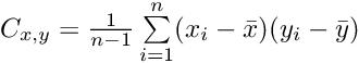
If we mean-center our data before, we can simplify the equation to the following:
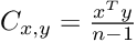
Once simplified, we can see that the calculation of the covariance is actually quite simple. It is just the dot product of two vectors containing data.
Now imagine, a dataset with three features x, y, and z. Computing the covariance matrix will yield us a 3 by 3 matrix. This matrix contains the covariance of each feature with all the other features and itself. We can visualize the covariance matrix like this:
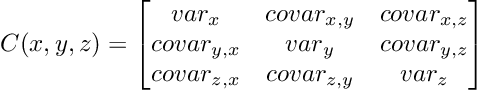
The covariance matrix is symmetric and feature-by-feature shaped. The diagonal contains the variance of a single feature, whereas the non-diagonal entries contain the covariance.
We already know how to compute the covariance matrix, we simply need to exchange the vectors from the equation above with the mean-centered data matrix.
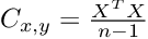
Once calculated, we can interpret the covariance matrix in the same way as described earlier, when we learned about the correlation coefficient.
Applying our knowledge
Now that we’ve finished the groundwork, let’s apply our knowledge.
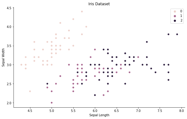
For testing purposes, we will use the iris dataset. The dataset consists of 150 samples with 4 different features (Sepal Length, Sepal Width, Petal Length, Petal Width)
Let’s take a first glance at the data by plotting the first two features in a scatterplot.
Our goal is to ‘manually’ compute the covariance matrix. Hence, we need to mean-center our data before. In order to do that, we define and apply the following function:
Note: We standardize the data by subtracting the mean and dividing it by the standard deviation.
Running the code above, standardizes our data and we obtain a mean of zero and a standard deviation of one as expected.
Next, we can compute the covariance matrix.
Note: The same computation can be achieved with NumPy’s built-in function numpy.cov(x).
Our covariance matrix is a 4 by 4 matrix, shaped feature-by-feature. We can visualize the matrix and the covariance by plotting it like the following:
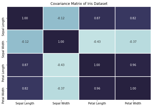
We can clearly see a lot of correlation among the different features, by obtaining high covariance or correlation coefficients. For example, the petal length seems to be highly positively correlated with the petal width, which makes sense intuitively — if the petal is longer it is probably also wider.
Conclusion
In this article, we learned how to compute and interpret the covariance matrix. We also covered some related concepts such as variance, standard deviation, covariance, and correlation.
The covariance matrix plays a central role in the principal component analysis. Implementing or computing it in a more manual approach ties a lot of important pieces together and breathes life into some linear algebra concepts.
Thank you for reading! Make sure to stay connected & follow me here on Medium, Kaggle, or just say ‘Hi’ on LinkedIn
Enjoyed the article? Become a Medium member and continue learning with no limits. I’ll receive a portion of your membership fee if you use the following link, at no extra cost to you.
References / Further Material:
- Implementing PCA From Scratch
- Mike X Cohen, PhD. Linear Algebra: Theory, Intuition, Code.


