Support Vector Machine: Kernel Trick; Mercer’s Theorem

Understanding SVM Series : Part 2

Prerequisite: 1. Knowledge of Support vector machine algorithm which I have discussed in the previous post. 2. Some basic knowledge of algebra.

In the 1st part of this series, from the mathematical formulation of support vectors, we have found two important concepts of SVM, which are

• SVM problem is a constrained minimization problem and we have learned to use Lagrange Multiplier method to deal with this.
• To find the widest road between different samples we just need to consider dot products of support vectors and the samples.

In the previous post of SVM, I took a simple example of samples that are linearly separable to demonstrate Support Vector Classifiers. What happens if we have a sample set like below ?

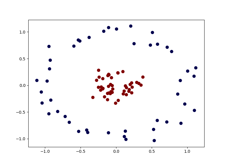
This plot is generated using the in built make_circlesdataset of sklearn.

import numpy as np 
import sklearn 
import matplotlib.pyplot as plt
from sklearn.datasets.samples_generator import make_circles

X,y = make_circles(90, factor=0.2, noise=0.1) 
#noise = standard deviation of Gaussian noise added in data. 
#factor = scale factor between the two circles

plt.scatter(X[:,0],X[:,1], c=y, s=50, cmap='seismic')
plt.show()

As you can understand that it is impossible to draw a line in this 2d plot which could separate the blue samples from the red ones. Is it still possible for us to apply SVM algorithm ?

What if we give this 2d space a bit of shaking and the red samples fly off the plane and appears separated from the blue samples ? Take a look !

Well it seems shaking the data samples indeed worked, and now we can easily draw a plane (instead of line as we have used before) to classify these samples. So what actually happened during shaking ?

When we don’t have linear separable set of training data like the example above (in real life scenario most of the data-set are quite complicated), the Kernel trick comes handy. The idea is mapping the non-linear separable data-set into a higher dimensional space where we can find a hyperplane that can separate the samples.

So it is all about finding the mapping function that transforms the 2D input space into a 3D output space. Or is it ? And what the heck is Kernel Trick ?

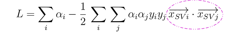
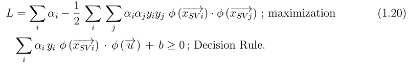
From the previous post about support vectors, we have already seen (please check to understand the mathematical formulation) that the maximization depends only on the dot products of support vectors,

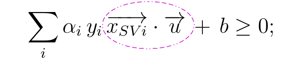
not only that, as the decision rule also depends on the dot product of support vector and a new sample

That means if we use a mapping function that maps our data into a higher dimensional space, then, the maximization and decision rule will depend on the dot products of the mapping function for different samples, as below -

And Voila!! If we have a function K defined as below

then we just need to know K and not the mapping function itself. This function is known as Kernel function and it reduces the complexity of finding the mapping function. So, Kernel function defines inner product in the transformed space.

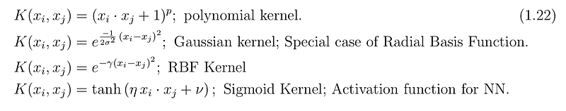
Let us look at some of the most used kernel functions

I have used Radial Basis Function kernel to plot figure 2, where mapping from 2D space to 3D space indeed helps us in classification.

Apart from this predefined kernels, what conditions determine which functions can be considered as Kernels ? This is given by Mercer’s theorem. First condition is rather trivial i.e. the Kernel function must be symmetric. As a Kernel function is dot product (inner product) of the mapping function we can write as below —

Mercer theorem guides us to the necessary and sufficient condition for a function to be Kernel function. One way to understand the theorem is —

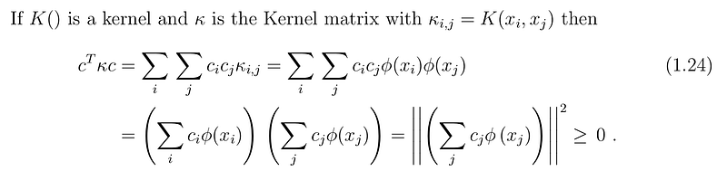
In other words, in a finite input space, if the Kernel matrix (also known as Gram matrix) is positive semi-definite then, the matrix element i.e. the function K can be a kernel function. So the Gram matrix merges all the information necessary for the learning algorithm, the data points and the mapping function fused into the inner product.

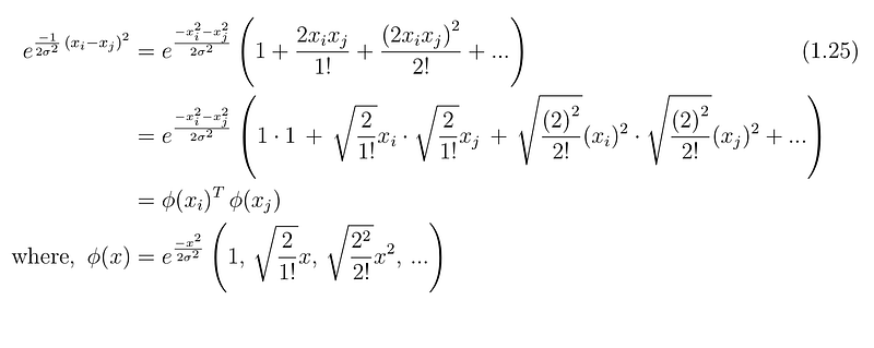
Let’s see an example of finding the mapping function from the kernel function and here we will use Gaussian kernel function

Tuning Parameter

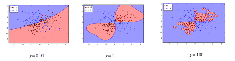
Since we have discussed about the non-linear kernels and specially Gaussian kernel (or RBF kernel), I will finish the post with intuitive understanding for one of the tuning parameters in SVM — gamma.

Looking at the RBF kernel we see that it depends on the Euclidean distance between two points, i.e. if two vectors are closer then this term is small. As the variance is always positive, this means for closer vectors, the RBF kernel is widely spread than the farther vectors. When gamma parameter is high the value of kernel function will be less, even for two close by samples, and, this may cause complicated decision boundary or give rise to over-fitting. You can read more on this in a different post by me.

Before we finish this discussion let’s recall what have we learn so far in this chapter —

1. Mapping data points from low dimensional space to a higher dimensional space can make it possible to apply SVM even for non-linear data sample.
2. We don’t need to know the mapping function itself, as long as we know the Kernel function ; Kernel Trick
3. Condition for a function to be considered as kernel function; Positive semi-definite Gram matrix.
4. Types of kernels that are used most.
5. How the tuning parameter gamma can lead to over fitting or bias in RBF kernel.

Hope you have enjoyed the post and, on the next chapter we will see some machine learning examples using SVM algorithm.

The complete math behind the SVM algorithm was discussed here:

For more on plotting and understanding support vector machine decision boundary, please check this post:

Stay Strong ! Cheers !!

If you’re interested in further fundamental machine learning concepts and more, you can consider joining Medium using My Link. You won’t pay anything extra but I’ll get a tiny commission. Appreciate you all!!

References:

1. “The Elements of Statistical Learning”; Hastie, T. et.al. ; amazon link
2. “Properties of Kernel ”; Berkley University; pdf.
3. “Kernels”; MIT lecture-notes.