Understanding Portfolio Diversification

Investing is all about risk management.

Disclaimer: The information contained in this blog post is strictly for educational and entertainment purposes only. This is also not an investment advice. All views expressed in this blog are my own and do not represent the opinions of any entity whatsoever with which I have been, am now, or will be affiliated.

____

In the recent times of markets tumbling, diversification can help to spread risk across different securities. Regardless of whether you are investing for the short or long term. Market movements that are abrupt and highly volatile can have a substantial impact on investments.

Diversification is the act of spreading one’s investments over a number of different securities to minimize risk and avoid putting all one’s eggs in one basket. It helps to reduce the volatility of an investment portfolio.

This is because while one security declines, another may rise and balance some of the losses suffered by the first, or it may decline less than the first.

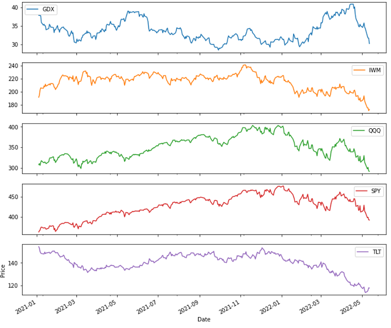
Let’s take a look at the performance of certain ETFs that track US stock indices (S&P500, Nasdaq 100, Russell 2000), government bonds and gold. The results cover the period between 2021–01–01 and 2022–05–13.

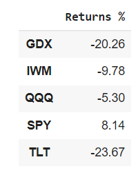
As we can see, each ETF presents a different return. Let’s imagine you invested $5000 in these five ETFs, $1000 into each one. At the end of the period you would be left with $4,491.30.

On the other hand, if you had put all $5000 into TLT, you have ended up with $3,816.50.

The results of the diversified portfolio also depends how correlated are the securities with each other. Correlation is the measure of how related two assets are. A high correlation between two assets indicates they move together. If you own stocks with a high correlation to each other, you are increasing your chances to lose money if one of them drops.

Let’s quickly look at the correlation among all of the above listed ETFs.

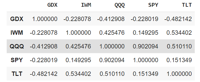
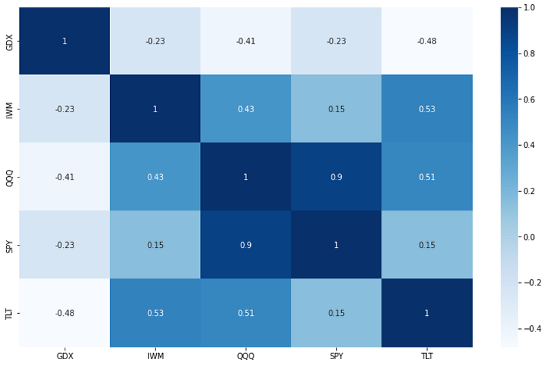
The higher the positive correlation between the securities, the closer the value is to +1. The higher the negative correlation between the securities, the closer the value is to -1. In contrast, the closer the value gets to 0, the less correlation exists.

For example, the correlation between TLT and QQQ is 0.51, which indicates a weaker correlation and hence a significant difference between their returns (-23.67% for TLT and -5.30% for QQQ).

Therefore, as can be seen, adding uncorrelated securities to the portfolio increases diversity even further.

Let’s take a look at some individual stocks before we wrap up this blog, focusing on some of the random S&P500 stocks: Apple (APPL), Amazon (AMZN), Tesla (TSLA).

Returns & Correlation:

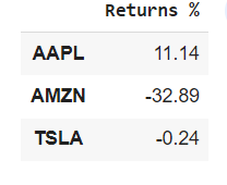
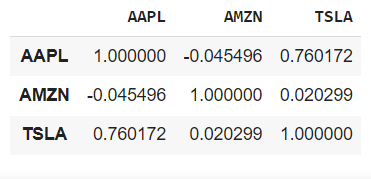
In this case, I believe the diversification message is even much more compelling.

Diversification can be used in any sort of portfolio, including options portfolios.

Thanks for reading!

Python code used for this blog 

#importing relevant packages 

import yfinance as yf
import pandas as pd
import seaborn as sns
import matplotlib.pyplot as plt

#downloading data 

tickers = ["SPY","QQQ","IWM", "GDX", "TLT"]
df =yf.download(tickers,  start = "2021-01-01" , end = "2022-05-13")

# calculating returns 

returns = round(((df['Adj Close'].iloc[-1,:] - df['Adj Close'].iloc[0,:]) / df['Adj Close'].iloc[0,:])*100, 2)

# saving returns into dataframe

df2 = pd.DataFrame(returns)
df2.rename(columns = {0 : 'Returns %'}, inplace = True)

# plotting the performance of each ETF 

df["Adj Close"].plot(subplots=True, figsize=(12, 11));
plt.legend(loc='best')
plt.xlabel('Date')
plt.ylabel('Price')
plt.show()

#calculating correlation among ETFs 

corr = df['Adj Close'].corr(method='pearson')

#visualizing correlation 

plt.figure(figsize=(13, 8))
sns.heatmap(corr, annot=True, cmap='Blues')
plt.figure()

##Analyzing AMZN, TSLA and AAPL stocks

tickers2 = ["AMZN","TSLA","AAPL"]
df2 =yf.download(tickers2,  start = "2021-01-01" , end = "2022-05-13")

returns2 = round(((df2['Adj Close'].iloc[-1,:] - df2['Adj Close'].iloc[0,:]) / df2['Adj Close'].iloc[0,:])*100, 2)

df3 = pd.DataFrame(returns2)
df3.rename(columns = {0 : 'Returns %'}, inplace = True)

corr2 = df2['Adj Close'].corr(method='pearson')

Subscribe to DDIntel Here.

Visit our website here: https://www.datadriveninvestor.com

Join our network here: https://datadriveninvestor.com/collaborate