
Understanding Matplotlib in 6 Code snippets
Matplotlib is a go-to library in python for data visualization. Have you explored all functions that this library offers? If not, let me help you!

I work as an Applied scientist at Amazon. Believe me or not, I don’t recollect any week in which I haven’t used this library for my work. Sometimes we need to visualize data for our understanding, and sometimes visualizations are required in presentations/documents. Hence depending on the need, we also have to worry about the intuition and beautification of visualization. Now, matplotlib, my friends, is my go-to library for all these tasks. In this blog, we will understand how to use matplotlib to plot the following variations:
- Plot a normal graph with an array of continuous data
- Plot categorical variable
- Plot graph to find the relation between two variables using scatter plot
- Plot graphs with the different formatting style
- Create figures comprising of multiple graphs — One graph with multiple curves or different graphs having different curves
- Work with text annotation in graphs.
The above is not an exhaustive list, but they should be good enough to understand the library. Let’s start!!!
Normal graph with an array of continuous data
One of the most straightforward use cases is understanding the behavior of loss with epochs/iteration while training a machine learning model.
import matplotlib.pyplot as plt
import numpy as np
loss = np.array([1, 0.95, 0.92, 0.89, 0.83, 0.76, 0.70, 0.63, 0.54, 0.48])
epochs = np.array(list(range(10)))plt.plot(loss, epochs)
plt.show()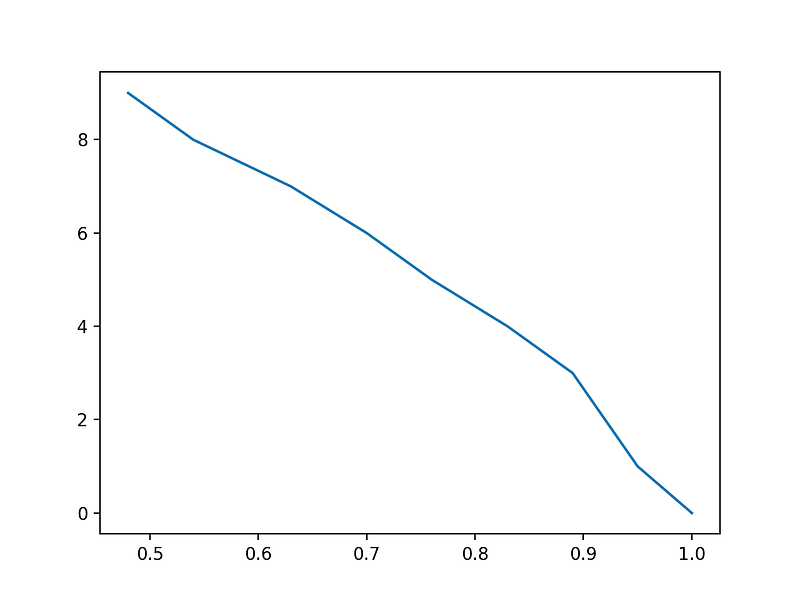
Yeah, I know the above graph looks pretty standard. Don’t worry, we will beautify it in the “Formatting styles” section.
Plot categorical variables/data
First of all, what are categorical variables? These variables take up discrete and finite numbers of values. For example, in a classification task, the variable describing the classes is a categorical variable. One tangible example is considering an image classification problem where we have to classify if the image has a dog (1) or not (0). Then this variable representing the number of images that had a dog present or not is a categorical variable. Such variables can be represented, say, using bar graphs or pie charts.
Bar graph-:
import matplotlib.pyplot as plt
import numpy as np
class_variable = ["dog", "cat", "cow", "fish"]
number_of_image = [10, 15, 8, 20]
plt.bar(class_variable, number_of_image)
plt.show()Pie Chart-:
import matplotlib.pyplot as plt
import numpy as np
class_variable = ["dog", "cat", "cow", "fish"]
number_of_image = [10, 15, 8, 20]
plt.pie(number_of_image, labels = class_variable)
plt.show()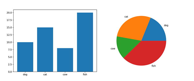
Plot graph to find the relation between two variables using scatter plot
As you might have guessed, a scatter plot is used to find the relation between two variables. Here we visualize how a change in one variable affects another variable, or in other words, we try to understand the correlation between two variables.
import matplotlib.pyplot as plt
import numpy as np
variable_a = np.array([5,7,8,7,2,17,2,9,4,11,12,9,6])
variable_b = np.array([99,86,87,88,111,86,103,87,94,78,77,85,86])plt.scatter(variable_a, variable_b)
plt.show()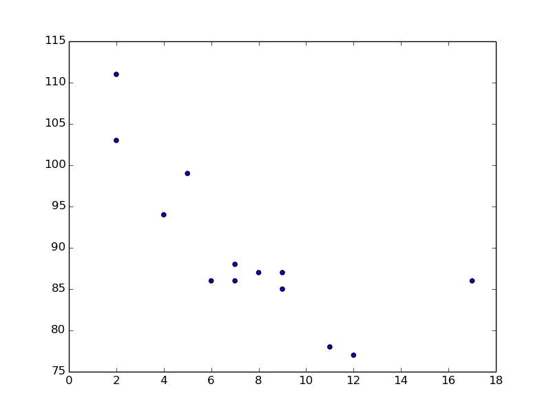
From the above graph, we can conclude that when variable_a increases, variable_b decreases.
Formatting Style of Plots
This is one of the important ones. Here we will see all kinds of beautification we can add to a plot. We will see how to add the following things here-:
- Axis label — Helps in describing what the x-axis and y-axis represent on the plot.
- Legend — Useful when we plot multiple plots in a graph. It tells which color represents which data in the plot.
- Title — Title of the plot
- Grid — Adding a grid in graph helps get better inference
- Color —Setting the color of the curve as per your requirement.
- Dashed lines — Setting if the curve should be a solid line or a dashed line
- Marker — Setting how to represent each data point
So a lot of new features are getting introduced. To understand the effect of each one, I have plotted multiple plots on different lines of code as commented in the snippet below.
Note — I have used only one type of marker or one type of color for illustration purposes. You can check out what other options are available for each type.
import matplotlib.pyplot as plt
import numpy as np
loss = np.array([1, 0.95, 0.92, 0.89, 0.83, 0.76, 0.70, 0.63, 0.54, 0.48])
epochs = np.array(list(range(10)))
plt.plot(loss, epochs, label="Loss Curve 1", linestyle="dashed", marker='*', color='red')#Plot 1
plt.xlabel("Epochs")
plt.ylabel("Loss") #Plot 2
plt.title("Loss - Epoch Curve")#Plot 3
plt.grid("on") #Plot 4
plt.legend()#Plot 5
plt.show()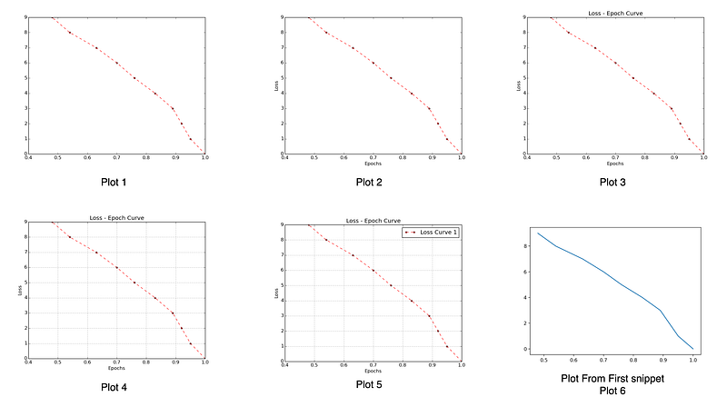
For comparison, I have also shown a plot from the first snippet (Plot 6). Now, for our understanding, Plot 6 is enough as we only need to see how the loss varies with each epoch. Still, for anyone new, Plot 5 is more appropriate to represent all the necessary information.
Creating a figure comprising of multiple graphs
When we need to plot multiple subplots, we can use the below snippet. I have also added different examples of formatting styles so that you can get more clarity.
import matplotlib.pyplot as plt
import numpy as np
t1 = np.arange(0.0, 5.0, 0.1)
t2 = np.arange(0.0, 5.0, 0.2)plt.figure()
plt.subplot(2,2,1)
plt.plot(t1, np.sin(2*np.pi*t1), color = 'black', marker='^', linestyle='solid')
plt.title("Sin Curve")
plt.grid("on")plt.subplot(2,2,2)
plt.plot(t2, np.tan(2*np.pi*t2), color = 'blue', marker='*', linestyle='dashed')
plt.title("Tan Curve")
plt.grid("on")plt.subplot(2,2,3)
plt.plot(t1, np.cos(2*np.pi*t1), color = 'green', marker='o', linestyle='dotted')
plt.title("Cos Curve")
plt.grid("on")plt.subplot(2,2,4)
plt.plot(t2, np.exp(t2), color = 'red', marker='*', linestyle='dashdot')
plt.title("Exponential Curve")
plt.grid("on")
plt.show()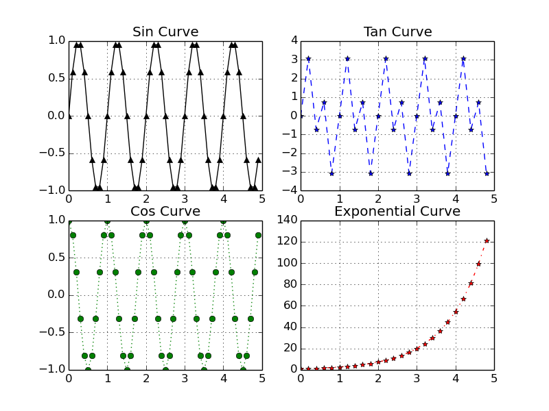
When multiple curves are required in the same plot then we can use the below snippet.
import matplotlib.pyplot as plt
import numpy as np
t1 = np.arange(0.0, 5.0, 0.1)
t2 = np.arange(0.0, 5.0, 0.2)plt.plot(t1, np.sin(2*np.pi*t1), color = 'black', marker='^', linestyle='solid', label = "Sin Curve")
plt.plot(t1, np.cos(2*np.pi*t1), color = 'green', marker='o', linestyle='dashed', label="Cos Curve")
plt.legend()
plt.grid("on")
plt.show()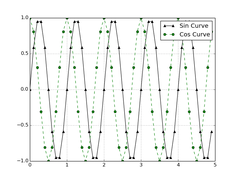
As we can see here, a legend is instrumental in visualizing which curve corresponds to which function, i.e., sin or cos.
Work with text annotation in graphs.
We can use test annotation to point out a particular point in the graph and describe what that point means. For example, I have annotated the maxima of the sin curve and the cos curve in the code below.
import matplotlib.pyplot as plt
import numpy as np
t1 = np.arange(0.0, 5.0, 0.1)
t2 = np.arange(0.0, 5.0, 0.2)plt.plot(t1, np.sin(2*np.pi*t1), color = 'blue', marker='^', linestyle='solid', label = "Sin Curve")
plt.plot(t1, np.cos(2*np.pi*t1), color = 'green', marker='o', linestyle='dashed', label="Cos Curve")
plt.annotate('Sin max', xy=(1.25, 1), xytext=(1.5, 1.15),
arrowprops=dict(facecolor='black', shrink=0.05),
)
plt.annotate('Cos max', xy=(2, 1), xytext=(2.25, 1.15),
arrowprops=dict(facecolor='black', shrink=0.05),
)
plt.ylim([-1.5, 1.5])
plt.legend()
plt.grid("on")
plt.show()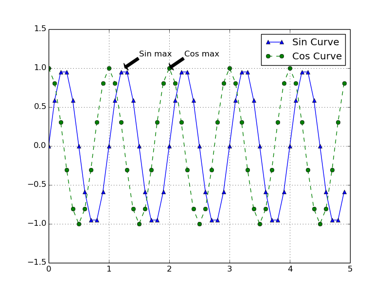
One more thing which I have added here is defining the limit of the y-axis. Similarly, you can change the limits for the x-axis.
Conclusion
Above are just a few examples using which I tried to cover as much breadth as possible. Now you can use multiple tools together to create a great visualization. If I have missed any important examples, please let me know so that I can add them here.
Thanks for dropping by!
Follow us on medium for more such content.
Become a Medium member to unlock and read many other stories on medium.


