Understanding core concepts in Apache Spark

Apache Spark is one of the most popular frameworks for big data processing nowadays. Its success is widely attributed to the 100x reduction in processing time with respect to MapReduce. This article summarizes some core concepts from Spark architecture that will allow you to fully take advantage of Spark’s capabilities.

1. Actions and transformations

The fundamental data structure of Apache spark is the RDD, which stands for Resilient Distributed Dataset. It is an immutable collection of data that is partitioned across the cluster’s nodes. Datasets and DataFrames APIs have been introduced since Spark 1.6 as abstractions on top of the RDD to handle more structured data, but the following concepts still apply.

A transformation is an operation that takes as input an RDD and produces another RDD as output (hence the immutable in the definition). Examples of transformations are map, select, filter, join etc.

Actions are actual computations that return a derived value, such as count or aggregate operations.

Transformations in Spark are lazy, actions are what actually trigger the execution. The list of actions and transformations performed on an RDD is stored internally in the lineage graph (also known as logical execution plan). This is part of what allows Spark to be robust to hardware failures, by reprocessing just a subset of the data in case of executor loss.

Spark distinguishes between narrow transformations and wide transformations. Narrow transformations are transformations for which the necessary data resides on one partition (e.g. select, filter, cast, etc.). For wide transformations, the data may come from several other partitions of a parent RDD (groupBy, sort, join, distinct, etc.)

2. Optimized Execution Planning

Starting from the code you have written, Spark’s Catalyst optimizer will perform a series of operations in order to compute and select the best Physical Execution Plan. It starts by analyzing the logical execution plan in order to identify possible optimizations, such as reordering or grouping filters together. A classic example of optimization is predicate pushdown, where an existing filtering operation is moved ahead of all other transformations in order to optimize the amount of data that needs to be processed.

Starting from the optimized logical plan, the Catalyst optimizer will generate several physical plans that describe how the various steps can be actually executed on the cluster. The best physical plan is selected using cost-based optimization that takes into consideration the execution time and the resources consumption. The whole process is a little bit more complex than what I have summarized here, so feel free to check out this article for a more comprehensive view of the process and some examples on how to make good usage of the explain function on your RDD.

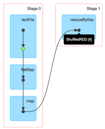
The selected physical plan contains the definition of the stages and the associated tasks, commonly known as the DAG (which stands for Direct Acyclic Graph). You can use the toDebugString function on your RDD to display the associated DAG or you can visualize it directly in the Spark History UI:

Explicitly caching your data in the code can prevent Spark from optimizing the execution. For instance, caching data before a filtering operation will eliminate the possibility of predicate pushdown. Things are obvious in this simple example but more complex applications require more attention.

3. Stage planning

During the execution planning phase Spark decides how the code will be split into stages, and the order in which they can be executed. To do so it starts from the lineage graph, working its way back from the action that triggers the computation. Whenever a wide transformation is encountered, which usually requires the data to be shuffled between the executors, it introduces a stage boundary.

A stage will end with a shuffle write step, which will cause some shuffle files to be written to disk, while the next stage will start with a shuffle read step. This is similar to what is happening when you explicitly cache the data.

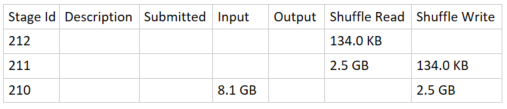
When looking at the details of the execution of a Spark job from the Spark History server, we can usually understand the order in which the various stages have been executed just by looking at the size of the corresponding Shuffle Read and Shuffle Write.

4. Partitioning

Spark splits the data across the cluster using partitions. The data in a partition exists on a single node on the cluster.

The repartition function can be used to increase or reduce the number of partitions but it is a wide transformation which involves shuffling all the data. The coalesce function can be used to reduce the number of partitions and it has the advantage of being a narrow transformation. However, it does not guarantee that the data is evenly balanced among the new partitions.

Fewer partitions allow work to be done in larger chunks with reduced shuffling overhead but there are physical limits to how much data a shuffle block can contain depending on the cluster’s cores configuration.

For a more comprehensive view of the partitioning options in Apache Spark you can check out this article.

I hope this post provided an overview of some of the main concepts in Apache Spark. For an example of using PySpark to process some data, you can check out this article. For an exemple of how to set up the Spark History Server and look at your DAG and the other metrics check out this post.