Understanding Conjugate Priors

Bayesian Approach to Machine Learning with PyMC3

In this post, I will give a comprehensive introduction to the concept of conjugate priors including some examples. Concept of conjugate prior is extremely useful because, conjugate priors reduce the Bayesian updating to only modifying some parameters in the prior distribution. They are also necessary to learn and understand Machine Learning from Bayesian approach. Jupyter notebook used for this post can be found in my GitHub (link below). What you may expect to learn from this post —

1. Definition of Conjugate Prior
2. Why it is relevant ?
3. Simple example to understand the concept.
4. Use PyMC3 as a tool for solving general Bayesian Inference.

So without any delay let’s begin:

Definition:

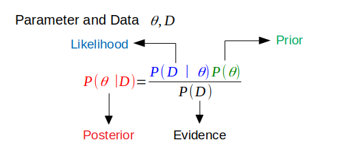
In Bayesian probability theory, if the posterior distribution is in the same family of the prior distribution, then the prior and posterior are called conjugate distributions, and the prior is called the conjugate prior to the likelihood function. Initially, you may think okay that’s cool but how exactly that helps us?

Why Conjugate Prior?

In Bayesian approach our goal is to obtain the posterior distribution. Calculation of evidence can cause a pain on the backside in real life problems. Let’s say, we are dealing with images and our objective is to generate a new image from a given set of images. It would be really difficult to model distribution of images, which is our P(D). Also, we can think of P(D) as a normalization constant and, it can be written as — — ∫ P(D|θ) P(θ) dθ. Imagine this integral in the context of a neural network where θs are the parameters, i.e. the weights of the network, and if it is a relatively deep network, there will be millions of θs. So the integral would be intractable. Conjugate prior is here to rescue us from this misery. We can obtain exact posterior distribution if our prior distribution (in case of the example above, it will be the distribution of weights) is conjugate prior for the likelihood function. Let’s see with a mischievous example:

As my friend Kitty has a not so friendly cat Nuo, patting her leads to either getting grumpy with probability p or start purring with probability (1-p). As this kind of behavior is not so well known to me, I assume a prior distribution on p with a Beta distribution, Beta(2, 2). If in one evening Nuo got grumpy 6 times and purred only 2 times, what are the parameters for posterior distribution over p? Each time patting Nuo can be considered as a single experiment with either of the two fixed outcomes. This is actually known as Bernoulli trial, similar to tossing a coin. As Beta distribution is conjugate to Bernoulli likelihood, we can already tell the posterior distribution would follow the Beta distribution (as shown in the derivation below). Let’s try to find the parameters…

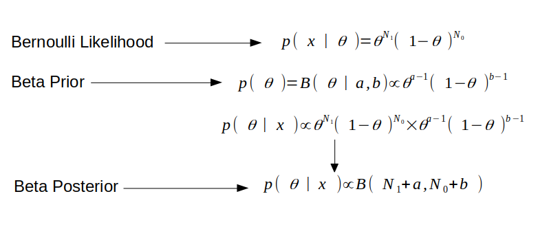
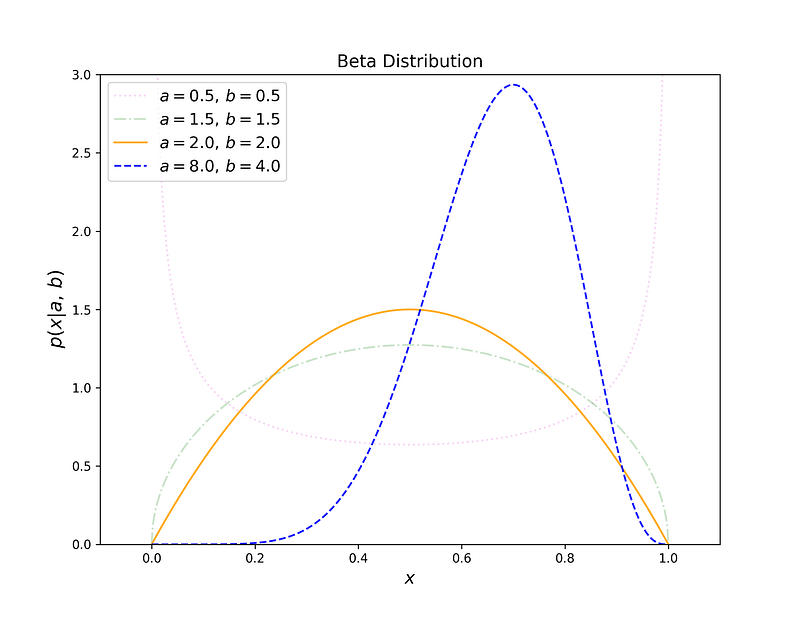
As we can see, for Bernoulli Likelihood we have outcome 1 for N1 times and 0 for N0 times. Selecting a Beta Prior with parameters a, b gives us Beta distribution with parameters (N1 + a, N0+b) as posterior. Thus, choosing conjugate prior helps us to compute the posterior distribution just by updating the parameters of prior distribution and, we don’t need to care about the evidence at all. Given our problem, we will have a posterior distribution which will be a Beta distribution with parameters (6+2, 2+2). Once we know the parameters of Beta distribution we can also calculate the Maximum a Posteriori which occurs at x = 0.7, as you can see in the figure below. Also, notice how the initial prior (Beta Distribution with parameters 2, 2) has changed to the updated posterior once we have used the likelihood. This is the key idea in Bayesian statistics, i.e., after seeing the data how our initial belief about the model has changed! For a detailed list of conjugate distributions check here.

Simple Example of Bayesian Update: Binomial and Beta

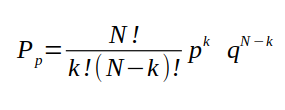
Let’s extend the previous silly example with a more realistic example where, we will use the fact that Binomial distribution is conjugate to the Beta distribution. For a single trial (ex: coin flip) the binomial distribution is equivalent to Bernoulli distribution. We will see how our knowledge of posterior updates as we gather more data. Let’s assume that we use a biased coin where our probability of success (heads) for Bernoulli trial is 0.4. We consider new observations as binomial distribution with k heads out of N trials. Starting with a simple Beta prior — β(1, 1) (which is equivalent to uniform prior), in the figure below, we see how more data helps us to update and reduce uncertainty of the posterior distribution.

Let’s see part of codes that I used to create the simple animation —

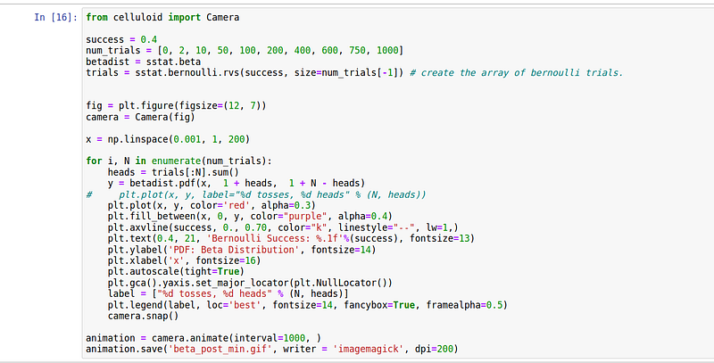
First, we create a numpy array of Bernoulli trials using scipy.stats.bernoulli.rvs and then count the number of success (heads) and failures. Based on this number, we update the Beta distribution starting from a uniform prior. Celluloid module was used for creating the matplotlib animation.

PyMC3 for Bayesian Modelling:

PyMC3 is a Python package for Bayesian statistical modeling built on top of Theano. It allows users to fit Bayesian models using various numerical methods including the Markov chain Monte Carlo (MCMC). Let’s start by building the coin flip model in PyMC3.

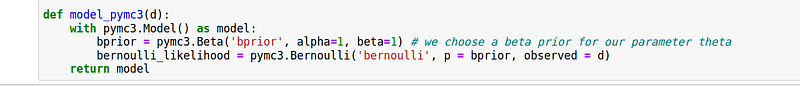
Here, we start with using Bernoulli likelihood, with the Beta prior with parameters (1, 1). In the observed variable of the Bernoulli function we will take the input data. It is a way of telling PyMC3 that we want to condition for the unknown given the known (observations).

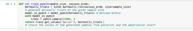
We create the Bernoulli trials and, this will be our input data. Given this observed data, we then tell PyMC3 to generate 15,000 samples from the posterior We return the generated samples and the observed data. With this, we are ready to call the function and generate samples —

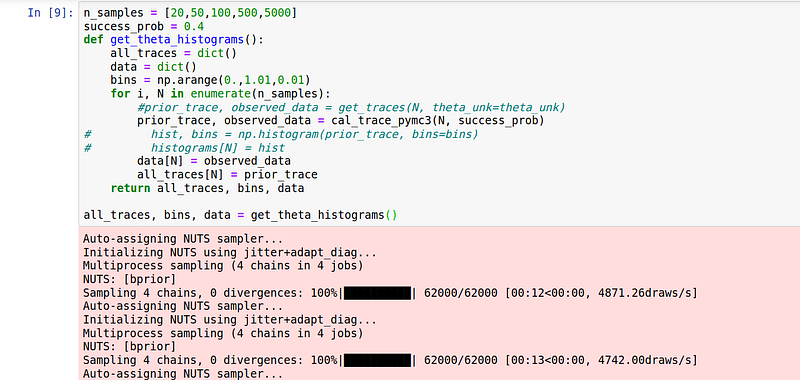
We create a list with number of observations (Bernoulli trials) and loop over this to collect all the generated samples and the corresponding observations and, store them in a dictionary. While executing this code-block you will see the number of samples generated using the No-U-Turn sampler(NUTS) is 62,000. The default sampler is NUTS in PyMC3 and it uses 4 cores (maximum number of CPUs) in parallel to create 15000 samples each. First 2000 samples (500 samples in each core) were used to tune the NUTS sampler which, later on will be eventually discarded. Check the documentation for more. Once the process of sample generation has finished, we can visualize the evolution of the posterior plot with increasing number of trials (observations) —

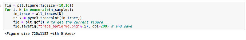
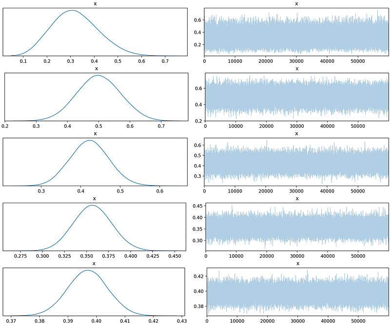
We can clearly see that with increasing number of trials, the uncertainty in the posterior distribution is becoming less. Let’s plot the histogram of the generated samples and compare with a true beta distribution (calculated using Scipy) —

Here, we have discussed conjugate prior and gone through some simple examples to solidify our understanding on why it is indeed important. Hopefully this will help you to at least get started with Bayesian Machine Learning.

Stay Strong and Cheers !

P.S: I covered another and probably the most important concept in Bayesian machine learning known as Latent variables and Expectation Maximization algorithm on a separate post.

Reference:

[1] Notes on Conjugate Priors — Professor M. Jordan; University of California, Berkeley.

[2] Link to my Notebook!