
Understanding BIRCH Clustering: Hands-On With Scikit-Learn
Unsupervised Learning — Clustering
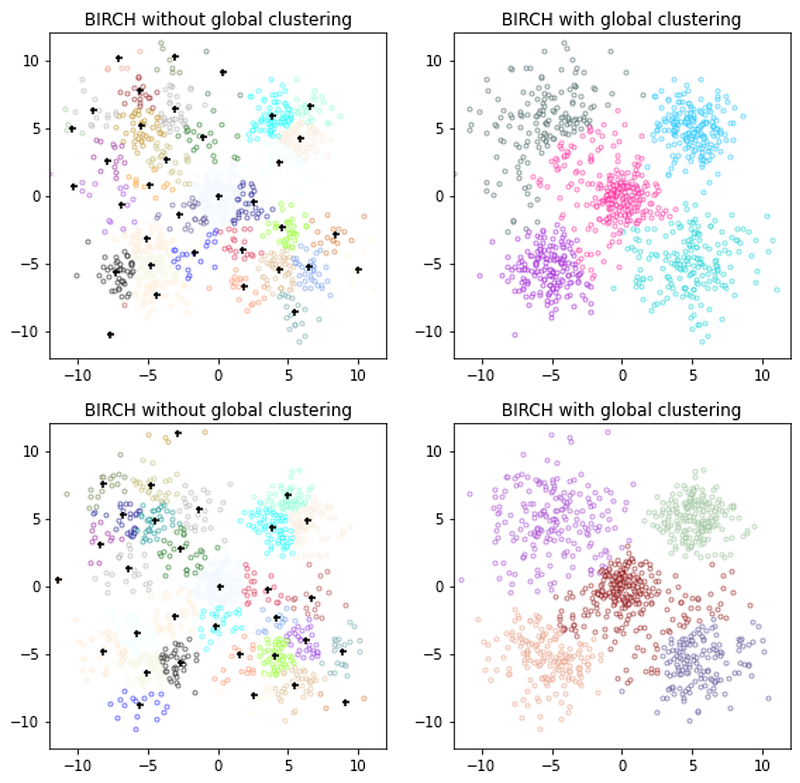
BIRCH → Balanced Iterative Reducing and Clustering using Hierarchies
The BIRCH algorithm is a solution for very large datasets where other clustering algorithms may not perform well. The algorithm creates a summary of the dataset by grouping similar observations (measured as euclidean distance) and providing a summary of the retained information.
BIRCH has two important attributes: Clustering Features (CF) and CF-Tree
The process of creating a CF tree involves reducing large sets of data into smaller, more concentrated clusters called Clustering Features (CF) entries. These entries are defined as a set of three values: the number of data points in the cluster (N), the linear sum of the data within a cluster (LS), and the squared sum of the data within the cluster (SS). The CF entries can also be made up of multiple other CF entries. Additionally, it is possible to further condense the initial CF into a smaller version — Global Clustering.
The CF tree is a type of tree that helps organize and manage clustering features while also holding important information about the data. This allows for hierarchical clustering to be performed without having to work with the full data.
The process of Global Clustering involves using a pre-existing clustering algorithm on the final sub-clusters located at the leaves of the CF-tree. A CF tree is a tree structure where each leaf node holds a sub-cluster, and every entry in the tree has a link to a child node, and the entry is made up of the combination of the entries of the child nodes. It is possible to improve the clusters by refining them further using two important parameters of the BIRCH algorithm:
threshold → when merging a new sample with the closest cluster, the radius of the resulting cluster should be smaller than a specific threshold. If it is not, a new cluster will be created. The threshold value is measured as the euclidean distance between two points and can be adjusted, with a lower threshold promoting more sub-clusters to be created, and a higher threshold promoting fewer clusters.
n_clusters → Is the number of clusters to be created. The final step of clustering involves treating the sub-clusters from the leaves as new samples and determining the number of clusters. The user can choose the number of clusters in the final clustering structure, or, if the value is set to ‘None’, this final step is not performed and the sub-clusters are returned as they are.
So, when should we run BIRCH with and without Global Clustering?
Without Global Clustering
→ To run BIRCH without global clustering, we set ‘n_clusters= None’. This means that the algorithm will only return the results of the initial CF tree.
→ When the BIRCH algorithm is run without global clustering, it only forms clusters from the data points within a certain radius and does not consider the overall structure. This can be useful for identifying clusters that are relatively isolated from one another and for handling large datasets where the computational cost of global clustering may be prohibitive.
→ Running BIRCH without global clustering can provide a good starting point for understanding the local structure of the data, however, it may not be able to identify more complex patterns and relationships within the dataset that are only apparent from the global structure.
With Global Clustering
→ When the BIRCH algorithm is run with global clustering, it considers the overall structure of the entire dataset and forms clusters based on the similarity of the data points throughout the entire data.
→ This can be useful for identifying clusters that are more closely related, and for discovering patterns and relationships within the data that may not be apparent from the local clusters alone.
Running BIRCH With and Without Global Clustering
→ Running the BIRCH algorithm both with and without global clustering can provide a more comprehensive understanding of the structure of the dataset and lead to more accurate and informative results. It is also possible to run the BIRCH algorithm without global clustering, and then run a different clustering algorithm on the results of BIRCH to get more information and possibly different cluster results.
We will see examples of all these case solutions!
We will import some libraries we need to run this project. I am using Google Colab for this one.
import pandas as pd
import numpy as np
import seaborn as sns
import matplotlib.pyplot as plt
import matplotlib.colors as colors
from sklearn.cluster import Birch, MiniBatchKMeans
from time import time
from itertools import cycle
Once BIRCH is specially designed to handle large datasets, we will build a toy dataset that is large enough to show you the capabilities of BIRCH. We will also time our code, so we can see the differences. The code I am using in this example is adapted from the Sci-Kit Learn working examples. Let’s now build a toy dataset. Our dataset will have 2 features (variables), and 10000000 entries.
# Set the number of samples and features
n_samples = 10000000
n_features = 2

# Create an empty array to store the data
data = np.empty((n_samples, n_features))

# Generate random data for each feature
for i in range(n_features):
    data[:, i] = np.random.normal(size=n_samples)

# Create 5 clusters with different densities and centroids
cluster1 = data[:2000000, :] + np.random.normal(size=(2000000, n_features), scale=0.5)
cluster2 = data[2000000:4000000, :] + np.random.normal(size=(2000000, n_features), scale=1) + np.array([5,5])
cluster3 = data[4000000:6000000, :] + np.random.normal(size=(2000000, n_features), scale=1.5) + np.array([-5,-5])
cluster4 = data[6000000:8000000, :] + np.random.normal(size=(2000000, n_features), scale=2) + np.array([5,-5])
cluster5 = data[8000000:, :] + np.random.normal(size=(2000000, n_features), scale=2.5) + np.array([-5,5])

# Combine the clusters into one dataset
X = np.concatenate((cluster1, cluster2, cluster3, cluster4, cluster5))

# Plot the data
plt.scatter(X[:, 0], X[:, 1])
plt.show()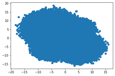
Now we will build two BIRCH models, one without global clustering and another with global clustering:
# Use all colors that matplotlib provides by default.
colors_ = cycle(colors.cnames.keys())

fig = plt.figure(figsize=(12, 4))
fig.subplots_adjust(left=0.04, right=0.98, bottom=0.1, top=0.9)

# Compute clustering with BIRCH with and without the final clustering step
# and plot.
birch_models = [
    Birch(threshold=1.7, n_clusters=None),
    Birch(threshold=1.7, n_clusters=5),
]
final_step = ["without global clustering", "with global clustering"]


for ind, (birch_model, info) in enumerate(zip(birch_models, final_step)):
    t = time()
    birch_model.fit(X)
    print("BIRCH %s as the final step took %0.2f seconds" % (info, (time() - t)))

    # Plot result
    labels = birch_model.labels_
    centroids = birch_model.subcluster_centers_
    n_clusters = np.unique(labels).size
    print("n_clusters : %d" % n_clusters)

    ax = fig.add_subplot(1, 3, ind + 1)
    for this_centroid, k, col in zip(centroids, range(n_clusters), colors_):
        mask = labels == k
        ax.scatter(X[mask, 0], X[mask, 1], c="w", edgecolor=col, marker=".", alpha=0.5)
        if birch_model.n_clusters is None:
            ax.scatter(this_centroid[0], this_centroid[1], marker="+", c="k", s=25)
    ax.set_ylim([-12, 12])
    ax.set_xlim([-12, 12])
    ax.set_autoscaley_on(False)
    ax.set_title("BIRCH %s" % info)

plt.show()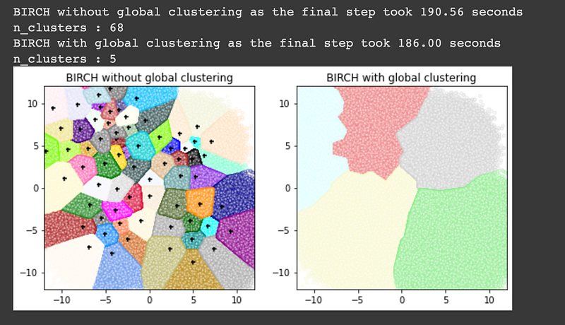
As you can see, the BIRCH model without global clustering returned 68 clusters, and the model with global clustering returned 5 clusters, however, the number of clusters in global clustering was specified by me, and you can try a different number.
As we learned before, we can also use BIRCH without global clustering, and then apply a different algorithm to the CF-tree. We will see an example where we will apply the K-Means algorithm after the BIRCH without global clustering:
from sklearn.cluster import KMeans

# Use all colors that matplotlib provides by default.
colors_ = cycle(colors.cnames.keys())

fig = plt.figure(figsize=(12, 4))
fig.subplots_adjust(left=0.04, right=0.98, bottom=0.1, top=0.9)

# Compute clustering with BIRCH with and without the final clustering step
# and plot.
birch_models = [
    Birch(threshold=1.7, n_clusters=None),
    KMeans(n_clusters=5),
]
final_step = ["without global clustering", " and K-means clustering"]


for ind, (birch_model, info) in enumerate(zip(birch_models, final_step)):
    t = time()
    birch_model.fit(X)
    print("BIRCH %s as the final step took %0.2f seconds" % (info, (time() - t)))

    # Plot result
    labels = birch_model.labels_
    #centroids = birch_model.subcluster_centers_
    n_clusters = np.unique(labels).size
    print("n_clusters : %d" % n_clusters)

    ax = fig.add_subplot(1, 3, ind + 1)
    for this_centroid, k, col in zip(centroids, range(n_clusters), colors_):
        mask = labels == k
        ax.scatter(X[mask, 0], X[mask, 1], c="w", edgecolor=col, marker=".", alpha=0.5)
        if birch_model.n_clusters is None:
            ax.scatter(this_centroid[0], this_centroid[1], marker="+", c="k", s=25)
    ax.set_ylim([-12, 12])
    ax.set_xlim([-12, 12])
    ax.set_autoscaley_on(False)
    ax.set_title("BIRCH %s" % info)

plt.show()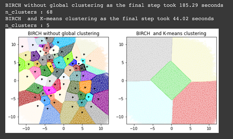
You can see that the K-Means algorithm took 44 seconds to run. The resulting clusters are also different from the BIRCH with global clustering. As we have learned, the BIRCH algorithm can be used before a different algorithm is applied to reduce computational costs. If we run K-Means without previous BIRCH, we can see that K-Means take longer time to run:
# Use all colors that matplotlib provides by default.
colors = ["o.", "r.", "b.", "y.", "c."]

fig = plt.figure(figsize=(12, 4))
fig.subplots_adjust(left=0.04, right=0.98, bottom=0.1, top=0.9)

# Compute clustering with BIRCH with and without the final clustering step
# and plot.
kmean = KMeans(n_clusters=5)
final_step = [""]


#for ind, (kmean, info) in enumerate(zip(kmean, final_step)):
 #   t = time()
kmean.fit(X)
print("K-Means %s as the final step took %0.2f seconds" % (info, (time() - t)))

# Plot result
labels = kmean.labels_
#centroids = birch_model.subcluster_centers_
n_clusters = np.unique(labels).size
print("n_clusters : %d" % n_clusters)

ax = fig.add_subplot(1, 3, ind + 1)
for this_centroid, k, col in zip(centroids, range(n_clusters), colors_):
    mask = labels == k
    ax.scatter(X[mask, 0], X[mask, 1], c="w", edgecolor=col, marker=".", alpha=0.5)
    if kmean.n_clusters is None:
        ax.scatter(this_centroid[0], this_centroid[1], marker="+", c="k", s=25)
ax.set_ylim([-12, 12])
ax.set_xlim([-12, 12])
ax.set_autoscaley_on(False)
ax.set_title("K-Means %s" % info)

plt.show()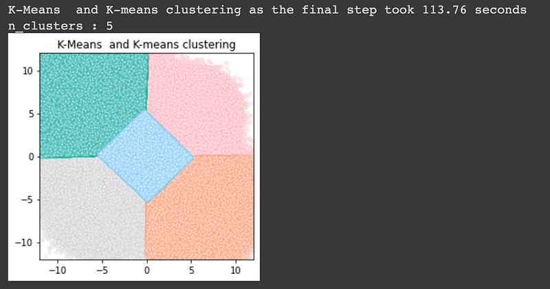
K-Means without previous BIRCH took 114 seconds to run versus the 44 seconds needed when previous BIRCH is applied.
Thank you for reading! Don’t forget to subscribe to receive notifications about my future publications.
If: you liked this article, don’t forget to follow me and thus receive all updates about new publications.
Else If: you want to read more on the topic, you can buy my book “Data-Driven Decisions: A Practical Introduction to Machine Learning” which will give you all the information you need to start with Machine Learning. It will cost you only a coffee, and give me a small tip!
Else: Thank you!


