Understanding Affinity Propagation Clustering: Hands-On with SciKit-Learn

Unsupervised Learning — Clustering

Affinity Propagation is a relatively recent model, first published in 2007 by Brendan Frey and Delbert Dueck. The model is a little complex in terms of resource consumption, as it requires our machines to perform several operations, but I will try to explain it to you in simple and plain English.

• The Affinity Propagation algorithm starts by considering data points that can be exemplars to form clusters. All data points are candidates to be ‘exemplar datapoints’.
• All ‘exemplar datapoints’ are compared to other data points, called ‘target datapoints’, to find how similar they are.
• The ‘target datapoints’ return to ‘exemplar datapoints’ if they are still available to associate. Otherwise, the ‘target datapoints’ may have already been associated with other ‘exemplar datapoints’ with whom they have higher affinity.
• The ‘exemplar datapoints’ respond to ‘target datapoints’ with an updated similarity.
• This dance continues until all data points are integrated into a cluster.

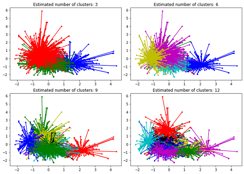
The Affinity Propagation algorithm does not require the researcher to specify the number of clusters, which means this algorithm is optimal for problems where we don’t know the ideal number of clusters. However, there is a way to control the number of clusters.

The PREFERENCE value:

The preference value should be used to control the number of clusters but does not correspond exactly to the number of clusters. A lower preference value (usually a negative number) will return fewer classes, while higher preference values will return more clusters in the model.

How do we control the number of clusters in the model?

We need to run the model several times with different preference values until we find a model with the desired number of clusters.

Let’s see a practical example:

We will use the wine dataset that can be downloaded from Kaggle. All code presented here was run on Google Colab.

#Import libraries:
import pandas as pd
import numpy as np
import seaborn as sns
import matplotlib.pyplot as plt

Now we will load and check the database:

#Load and read data frame:
df = pd.read_csv('wine.csv')
df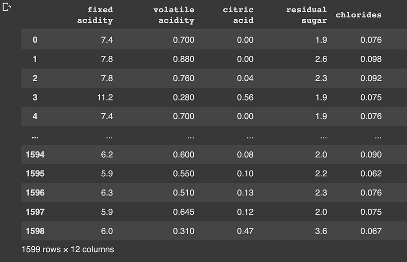

We have 1599 observations and 12 features. We will check if all our features are numeric:

#Check all features are numeric:
df.dtypes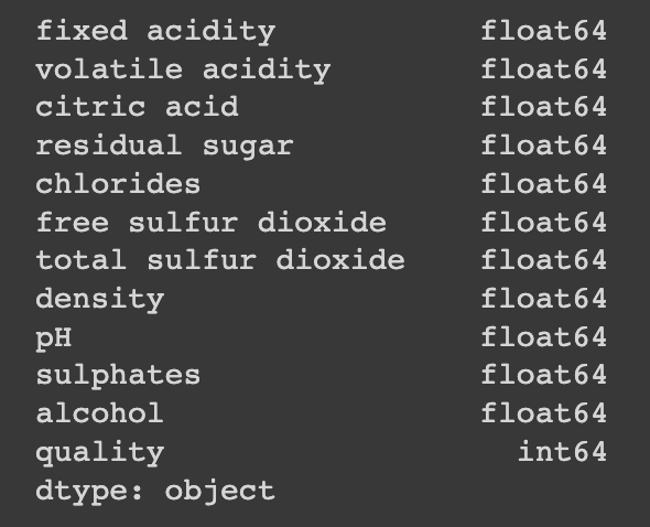

Now we will define and transform our dataset using the Standard Scaler function:

#Define X as numpy array:
X = np.array(df)

from sklearn.preprocessing import StandardScaler

#Transform X:
scaler = StandardScaler()
X = scaler.fit_transform(X)

It is time to build our model, so let’s import the necessary packages:

from sklearn.cluster import AffinityPropagation
from sklearn import metrics

And now we can build the model and fit our data. Take close attention to the preference value:

#Fit the model:
af = AffinityPropagation(preference=-1800, random_state=0).fit(X)
cluster_centers_indices = af.cluster_centers_indices_
labels = af.labels_
n_clusters_ = len(cluster_centers_indices)

#Print results:
print(labels)

#Print number of clusters:
print(n_cluster_)

You can run this last part of the code several times while trying with different preference values. The last step is to build a graphical representation. The image you can see at the beginning of this article was obtained using this exact code while experimenting with different preference values.

import matplotlib.pyplot as plt
from itertools import cycle

plt.close("all")
plt.figure(1)
plt.clf()

colors = cycle("bgrcmykbgrcmykbgrcmykbgrcmyk")
for k, col in zip(range(n_clusters_), colors):
    class_members = labels == k
    cluster_center = X[cluster_centers_indices[k]]
    plt.plot(X[class_members, 0], X[class_members, 1], col + ".")
    plt.plot(
        cluster_center[0],
        cluster_center[1],
        "o",
        markerfacecolor=col,
        markeredgecolor="k",
        markersize=14,
    )
    for x in X[class_members]:
        plt.plot([cluster_center[0], x[0]], [cluster_center[1], x[1]], col)

plt.title("Estimated number of clusters: %d" % n_clusters_)
plt.show()

Thank you for reading! Don’t forget to subscribe to receive notifications about my future publications.

If: you liked this article, don’t forget to follow me and thus receive all updates about new publications.

Else If: you want to read more on the topic, you can buy my book “Data-Driven Decisions: A Practical Introduction to Machine Learning” which will give you all the information you need to start with Machine Learning. It will cost you only a coffee, and give me a small tip!

Else: Thank you!