Deep Learning

Simplifying Complex Text with Abstractive Summarization

A CNN news articles summarization case study

Linkedin profile & Github profile for code implementation.

Introduction to Text Summarization
Exploring the CNN Dataset
Data Cleaning Methodologies
Analytical Approaches to Text Data
Evaluation Metrics for Summarization
Preprocessing Techniques for Text Data
Establishing a Baseline Model
Attention layer
Introduction to the Coverage Mechanism
Pre-trained BERT for Summarization
Fine-tuning the T5 Model for Optimized Results
Model Analysis
Conclusion
References

1. Introduction to Text Summarization

Automatic summarization refers to the computational technique of condensing extensive data into a concise form while retaining the most crucial information from the original content.

Classification of Text Summarization: Text summarization can broadly be categorized into two methods: Extractive and Abstractive Summarization.

Extractive Summarization:

This approach directly identifies and extracts salient points or sentences from the source text.
The extracted content is then rearranged, and in some cases, minor grammatical adjustments are made to ensure coherence.
The essence of this method is to pull directly from the original without altering the core meaning or introducing new phrases. The resulting summary is a distilled version of the original content.

Abstractive Summarization:

Abstractive techniques, in contrast, generate a completely new summary, often introducing phrases or sentences not found in the source material.
This method leverages advanced linguistic and algorithmic techniques to interpret and capture the gist of the original content.
The resultant summary is not a mere extraction but a reinterpretation, providing a fresh and concise representation of the main ideas.
In essence, while extractive summarization focuses on selecting existing content, abstractive summarization aims to understand and then recreate the content in a condensed form.

2. Exploring the CNN Dataset

(Source: https://cs.nyu.edu/~kcho/DMQA/)

The CNN Dataset, available through the Digital Methods and Quantitative Analysis (DMQA) project at New York University, provides an extensive collection of journalistic content. Originating from CNN, a globally renowned news network, this dataset encompasses a wide array of topics, reflecting the network’s comprehensive news coverage over various periods. With approximately 90,000 documents in its vault, the richness of the dataset is further underscored by its structure: each document is not just limited to the main news story. It also features highlights, and brief segments that encapsulate the central themes and significant points of the articles, enabling researchers and data enthusiasts to grasp the essence of the stories at a glance. Such a format is especially beneficial for tasks like text summarization, where identifying key points is paramount.

file = open('Data/cnn/stories' + '/' + '000c835555db62e319854d9f8912061cdca1893e.story', encoding=utf-8)text = file.read() 
file.close() 
text

3. Data cleaning

Working with raw and unstructured data can be challenging, especially when aiming for accurate text summarization. The stories in our dataset are riddled with unwanted characters, symbols, and contractions. To address this and ensure the efficacy of our summarization algorithms, a structured data preprocessing routine is paramount.

a) Extracting summary from the articles:

def loading_articles(file_name): 
    file = open(file_name, encoding='utf-8')
    text = file.read()
    file.close()
    return text

def split_story(doc):
    index = doc.find('@highlight')
    story, highlights = doc[:index], doc[index:].split('@highlight')
    highlights = [h.strip() for h in highlights if len(h) > 0]
    return story, highlights

def split_story(doc):
    index = doc.find('@highlight')
    story, highlights = doc[:index], doc[index:].split('@highlight')
    highlights = [h.strip() for h in highlights if len(h) > 0]
    return story, highlights

The summary is labeled in the article after ‘@highlight.’ The above function will extract a summary from the articles also separate story articles and summary

b) Expanding the contraction words:

A contraction is a word made by shortening or combining two words. Words like can’t (can + not), don’t (do + not), and I’ve (I + have) are all contractions. As a cleaning step, we expand all those contractions with the following function.

def decontracted(phrase): 
    phrase = re.sub(r"won't", "will not", phrase) 
    phrase = re.sub(r"can\'t", "can not", phrase)  
    phrase = re.sub(r"n\'t", " not", phrase)  
    phrase = re.sub(r"\'re", " are", phrase)  
    phrase = re.sub(r"\'s", " is", phrase)  
    phrase = re.sub(r"\'d", " would", phrase)  
    phrase = re.sub(r"\'ll", " will", phrase)  
    phrase = re.sub(r"\'t", " not", phrase)  
    phrase = re.sub(r"\'ve", " have", phrase)  
    phrase = re.sub(r"\'m", " am", phrase)  
    return phrase

c) Removing unwanted symbols :

Token ‘(CNN)’ is present at the start of every article which doesn’t make any sense. so that token from the document and also ‘$%^&*#’ symbols are removed.

article_text=[]for i in CNN.article.values:tt=re.sub(r'\n',' ', i)
    tt=re.sub(r"([?!¿])", r" \1 ", tt)
    tt=decontracted(tt)
    tt = re.sub('[^A-Za-z0-9.,]+', ' ', tt)
    tt = tt.lower()
article_text.append(tt)

After cleaning all the text it is converted to lowercase.

4.Text data analysis

a)Article lengths:

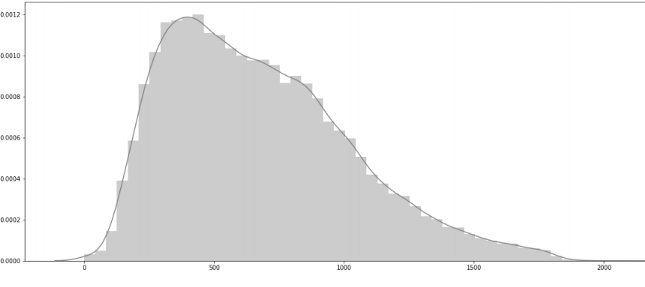
Article length distribution

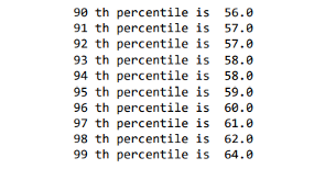
Most of the articles are of length 800 and distribution looks right-skewed and let’s check length percentile values from 90–99

import numpy as np 
b = [i for i in range(90,100)] 
for i in b:  
    print(i,'th percentile is ', np.percentile(art_len, i))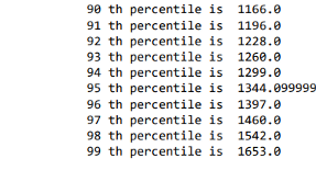

95th percentile article-length confidence interval

percentiles_95=[]
for i in range(0,200):
    samples=sample(summ_len,500)
    k=np.percentile(samples, 95)
    percentiles_95.append(k)
    mean = np.round(mean(percentiles_95),3)
    std = np.round(stdev(percentiles_95),3)
    left_limit = np.round(mean - 2*(std/np.sqrt(sample_size)), 3)     
    right_limit = np.round(mean + 2*(std/np.sqrt(sample_size)), 3)   print("95% of CI for MSE=",[left_limit,right_limit])

b) summary lengths:

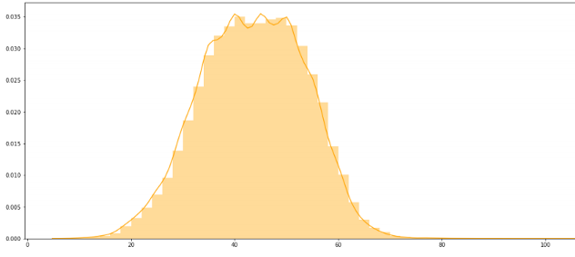
summary length distribution

It seems like most of the summaries have length 35–55 words. Looks interesting.. let’s explore percentile values.

95th percentile summary-length confidence interval

percentiles_95=[]
for i in range(0,200):
    samples=sample(summ_len,500)
    k=np.percentile(samples, 95)
    percentiles_95.append(k)
    mean = np.round(mean(percentiles_95),3)
    std = np.round(stdev(percentiles_95),3)
    left_limit = np.round(mean - 2*(std/np.sqrt(sample_size)), 3)     
    right_limit = np.round(mean + 2*(std/np.sqrt(sample_size)), 3)   print("95% of CI for MSE=",[left_limit,right_limit])

Let’s dig further more and find which words are more frequent in summary.

c)Word cloud for summary words:

Here the size of each word indicates its frequency or importance. Significant textual data points can be highlighted using a word cloud.

One interesting thing we can observe here is verbs like ‘say’,’ said’,’ will’,’ may’ are more frequent in summaries.

As CNN article is an American news-based, words like ‘American’, ‘new york’, ‘united states’ have significant importance in the cloud.

d) Parts of speech tagging to summaries and articles:

import spacy
sum_pos=[]
nlp = spacy.load("en_core_web_lg")
for i in tqdm(data_cleaned.Summary.values):
    pos_tag=[]
    doc = nlp(i)
    for token in doc:
        pos_tag.append(token.pos_)
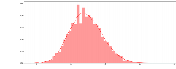
    sum_pos.append(pos_tag)

Noun percentages distribution

noun_percent=[]
for i in sum_pos:
    lent = i.count('NOUN')
    lentl = i.count('PROPN')
    noun=((lent+lentl)/len(i))*100
    noun_percent.append(noun)plt.figure(figsize=(20,8))sns.distplot(noun_percent,color='red');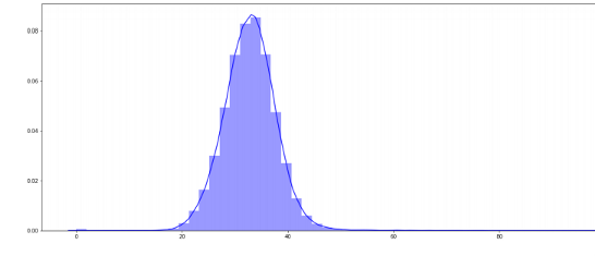

Nouns percentages Distribution summary and articles

Verb percentages distribution

verb_percent=[]for i in sum_pos:
    lent = i.count('VERB')
    verb=(lent/len(i))*100
    verb_percent.append(verb)
plt.figure(figsize=(20,8))
sns.distplot(verb_percent,color='red');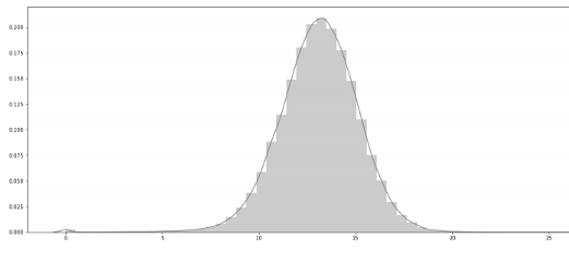

Verbs percentage distribution in summary and articles

e) Named_entities tagging:

The named entity is a real-world object, such as persons, locations, organizations, products, etc., that can be denoted with a proper name. It can be abstract or have a physical existence.

import spacy
from spacy import displacy
from IPython.core.display import display, HTML
nlp = spacy.load("en_core_web_lg")
doc2 = nlp(data_cleaned.Article.values[2])
displacy.render(doc2, style="ent", jupyter=True)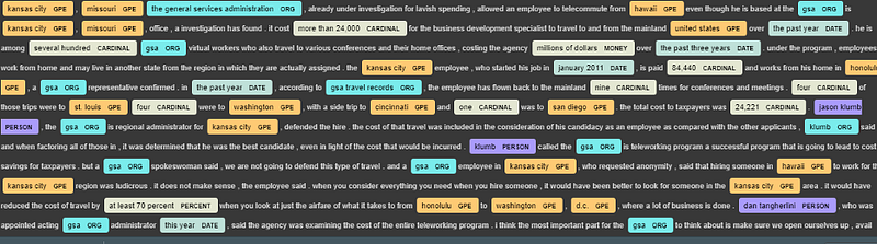

Article with named entities

f)Observations from the analysis:

1) Each summary has an average of 30 percent of nouns and 15 percent of verbs.

2) From the visualization of named entities, we can say that there is a high probability of considering a sentence containing the ORG entity as a summary. As the article has only two ‘org’ entities ‘GSA’ org entity selected in summary.

5. Evaluation metric

Summarization is a tough problem because the system has to understand the point of a text. This requires semantic analysis and grouping of the content using word knowledge.

Two general evaluation metrics used for summarization results are BLEU and ROGUE

a) BLEU Score is used to find the quality of text which has been predicted from one language to another.

BLEU stands for bilingual evaluation understudy

BLEU scores range from 0 and 1. If predicted and original text is a similar score close to 1 and vice-versa.

What is ROUGE?

To evaluate the goodness of the generated summary, the common metric in the Text Summarization space is called Rouge score.

ROUGE stands for Recall-Oriented Understudy for Gisting Evaluation.

It works by comparing an automatically produced summary or translation against a set of reference summaries (typically human-produced). It works by matching the overlap of n-grams of the generated and reference summary.

ROUGE-1 refers to the overlap of unigram (each word) between the system and reference summaries.

ROUGE-2 refers to the overlap of bigrams between the system and reference summaries.

ROUGE-L: Longest Common Subsequence (LCS) based statistics. The longest common subsequence problem takes into account sentence-level structure similarity naturally and identifies the longest cooccurring in sequence n-grams automatically.

ROUGE-n recall=40% means that 40% of the n-grams in the reference summary are also present in the generated summary.

For this model, I’m using the rogue score as an evaluation metric

6. Data Preprocessing

a) Replacing entities in text:

The named entity is a real-world object, such as persons, locations, organizations, products, etc., that can be denoted with a proper name. It can be abstract or have a physical existence. If we consider them as vocab perceptive most of them are categorized as rare words.

for i in range(len(cleaned_text)):
    doc1 = nlp(cleaned_text[i])
    c=(" ".join([t.text if not t.ent_type_ else t.ent_type_ for t in    doc1]))
    c=c.lower()
    short_text.append(c)doc2 = nlp(cleaned_summary[i])
    k=(" ".join([t.text if not t.ent_type_ else t.ent_type_ for t in    doc2]))
    k=k.lower()
    short_summary.append(k)

Let’s say there is an article about the person name ‘Johnathan Nolan’ if we didn’t see this name again in other articles, the article model can assume these names as rare words. But that word has a lot of importance in summary. So we are replacing entities in text.

Eg: ‘Johnathan Nolan directed web series in Netflix’ converted to ‘Person directed web series in gpe’

b)Handling OOV words :

Words that are present in train data and missing in test data are considered as out of vocabulary words.

what’s wrong with Keras Tokenizer(oov_token=’ukn’)?

If we use oov_token=’ukn’ in tokenizer it will replace all test tokens which are missing in training vocab. While testing we are giving untrained embedding to model as ‘unk’ is not trained. This will affect the model performance significantly.

So we have to include ‘ukn’ token in training, for that I am considering rare words in the training vocabs as ‘ukn’.

thresh=2
rare_word=[]for key,value in y_tokenizer.word_counts.items():
    if(value<thresh):
    rare_word.append(key)

Here I am considering my threshold value as two. This indicates if word frequency in the corpus is less than 2 then append those words as rare words.

tokenrare=[]
for i in range(len(rare_word)):
    tokenrare.append('ukn')
dictionary_1 = dict(zip(rare_word,tokenrare))
y_trunk=[]
for i in y_train:
    for word in i.split():
        if word.lower() in dictionary_1:
            i = i.replace(word, dictionary_1[word.lower()])
     y_trunk.append(i)

By using this code snippet I replace rare words in train documents with ‘unk’.This process helps to give better word embedding to rare words in train data as well as ‘unk’ character in test data.

c) Tokenizing and padding:

we are using the Keras tokenizer to tokenize words. After the tokenizer has been created, we then fit it on the training data then we will use it later to fit the testing data as well.

Then we need to do padding since every sentence in the text has not the same number of words, we can also define the maximum number of words for each sentence, if a sentence is longer then we can drop some words. Here we have the lines for padding as illustrated below:

y_tokenizer = Tokenizer(oov_token='ukn')
y_tokenizer.fit_on_texts(list(y_trunk)) 
y_tr_seq = y_tokenizer.texts_to_sequences(y_trunk)y_val_seq = y_tokenizer.texts_to_sequences(y_validatioin)zero upto maximum lengthy_tr = pad_sequences(y_tr_seq,maxlen=max_summary_len, padding='post')y_val = pad_sequences(y_val_seq, maxlen=max_summary_len, padding='post')y_voc = len(y_tokenizer.word_index) +1

d) Word Embeddings:

Word embeddings are techniques where single words are interpreted as real-valued vectors in a predefined vector space. Each word is mapped to one vector and the vector values are learned in a way that resembles a neural network.

These word embeddings are learned representation for text where words that have the same meaning have a similar representation. It is this approach to represent the words and documents that may be considered as one of the key breakthroughs of deep learning on challenging natural language processing problems.

The key to the approach is the idea of using a densely distributed representation for each word.

Here I am using pre-trained 100dim glove vectors.

embeddings_dictionary = dict()glove_file = open("/content/gdrive/My Drive/glove.6B.100d.txt", encoding="utf8")for line in glove_file:  
    records = line.split()  
    word = records[0]  
    vector_dimensions = np.asarray(records[1:], dtype='float32')               
    embeddings_dictionary [word] = vector_dimensions   glove_file.close()

7. Baseline model

I used a simple Encoder-Decoder model as the baseline model here is the architecture I used.

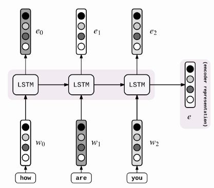
Encoder

encoder_inputs = Input(shape=(max_text_len,))enc_emb = Embedding(x_voc+1, 50,mask_zero=True, weights=[embedding_matrix_x] ,trainable=True)encoder = Bidirectional(LSTM(64, return_state=True))encoder_outputs, forward_h, forward_c, backward_h,  backward_c=encoder(enc_emb)state_h = Concatenate()([forward_h, backward_h])state_c = Concatenate()([forward_c, backward_c])

For Encoder, we can use the LSTM/GRU cells here I’m using bidirectional LSTM as the encoder. Which returns encoder_outputs, forward_h, forward_c, backward_h, backward_c .
Then concatenate forward and backward state and cell outputs which will be given to decoder as initial states.
An encoder takes the input sequence and encapsulates the information as the internal state vectors.

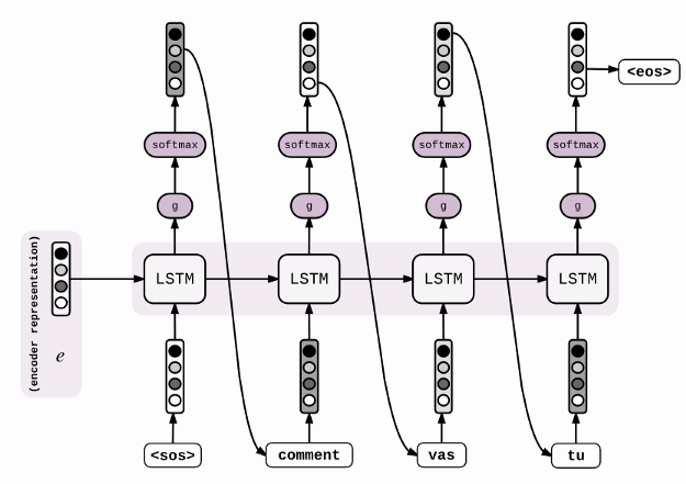
Decoder

decoder_inputs = Input(shape=(max_sum_len,)) #embedding layerdec_emb_layer = Embedding(y_voc+1, 50,mask_zero=True, weights=[embedding_matrix_y])dec_emb = dec_emb_layer(decoder_inputs)decoder_lstm = LSTM(128, return_sequences=True, return_state=True)decoder_output,decoder_state_h, decoder_state_c = decoder_lstm(dec_emb,initial_state=[state_h,state_c])dense layer decoder_dense = TimeDistributed(Dense(y_voc+1, activation='softmax'))decoder_outputs = decoder_dense(decoder_output)model1 = Model([encoder_inputs, decoder_inputs], decoder_outputs)

For the decoder, we are giving summaries as input and uses the teacher forcing techniques to train the model.

As shown in the decoder structure our first-time stamp input is ‘start’(y1) output of decoder LSTM cell given to dense layer of size summary vocab.

Then applying softmax to its results to give a probability distribution of vocab. We can pick words with the highest probability as the next word in the summary (say y2). This y2 is input for the next timestamp of LSTM.

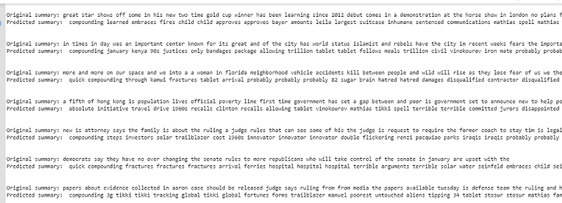
Predicted Summary:

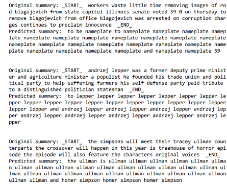
It was clear that the model is unable to predict the summary clearly and repeating the same words. Let’s check the model by adding the attention layer to it now.

8. Attention layer

Why Attention?

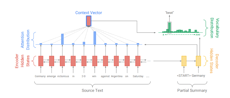
The standard seq2seq model is generally unable to accurately process long input sequences since only the last hidden state of the encoder RNN is used as the context vector for the decoder. On the other hand, the Attention Mechanism directly addresses this issue as it retains and utilizes all the hidden states of the input sequence during the decoding process. It does this by creating a unique mapping between each time step of the decoder output to all the encoder hidden states. This means that for each output that the decoder makes, it has access to the entire input sequence and can selectively pick out specific elements from that sequence to produce the output.

Therefore, the mechanism allows the model to focus and place more “Attention” on the relevant parts of the input sequence as needed.

Understanding the attention mechanism

When we think about the English word “Attention”, we know that it means directing your focus at something and giving greater notice. The Attention mechanism in Deep Learning is based on this concept of directing your focus, and it pays greater attention to certain factors when processing the data.

We’ll be using the same Encoder from the baseline model to produce hidden state/output for each input passed in. Instead of using only the hidden state at the final time step, we’ll be carrying forward all the hidden states produced by the encoder to the next step.

class additiveAttention(tf.keras.layers.AdditiveAttention): 
    def __init__(self,units):  
    super(additiveAttention,self).__init__()  
    self.units = units   
    self.W1 = Dense(units)  
    self.W2 = Dense(units)  
    self.V = Dense(1)  
    @tf.function  
    
    def call(self, keys):   
        query=keys[0]  
        values=keys[1]  
        ht_with_time_axis = tf.expand_dims(values, axis=1)score = self.V(tf.nn.tanh(self.W1(ht_with_time_axis) +      self.W2(query)))  
        attention_weights = tf.nn.softmax(score, axis=1)    
        context_vector = attention_weights * query  
        context_vector = tf.reduce_sum(context_vector, axis=1)return context_vector, attention_weights

Calculating Alignment Score :

To calculate At Alignment Score at decoder time step t we will be considered decoder hidden states of (t-1) and encoder hidden states.

from above code

query shape(encoder outputs) == (batch size,max_length,hidden size) values shape(decoder hidden at(t-1)) == (batch size,hidden size)

scorealignment=Wcombined⋅tanh(Wdecoder⋅Hdecoder+Wencoder⋅Hencoder)

Context Vector:

Attention_weights=softmax(scorealignment)

context_vector=Attention_weights*query

The context vector we produced will then be concatenated with the previous decoder output. It is then fed into the decoder RNN cell to produce a new hidden state and the process repeats itself. The final output for the time step is obtained by passing the new hidden state through a dense layer, which acts as a classifier to give the probability scores of the next predicted word.

Our attention model is trying to predict words but the overall predicted summary doesn’t make any sense and many words are repeating. To avoid repetition of words I am adding coverage mechanism to my model. let’s check how it works.

9. Coverage Mechanism

Repetition is a common problem for sequence-to-sequence models and is especially pronounced when generating multi-sentence text.

In this coverage mechanism, we use a coverage vector ct, which is the sum of attention distributions over all previous decoder timesteps.

Intuitively, ct is a distribution over the source document words that represents the degree of coverage that those words have received from the attention mechanism so far. Note that c0 is a zero vector because, on the first timestep, none of the source document has been covered

we add this coverage vector in the attention mechanism while finding alignment score as we have seen in the above section.

class additiveAttention(tf.keras.layers.AdditiveAttention):  
    def __init__(self, hidden_units,is_coverage=False):   
        super().__init__()   
        self.Wh = tf.keras.layers.Dense(hidden_units) 
        self.Ws = tf.keras.layers.Dense(hidden_units)
        self.wc = tf.keras.layers.Dense(1)
        self.V = tf.keras.layers.Dense(1)  
        self.coverage = is_coverage  
        
        if self.coverage is False:  
             self.wc.trainable = Falsedef call(self,keys):    
        value=keys[0]  
        query=keys[1]  
        ct=keys[2]    
        value = tf.expand_dims(value, 1)
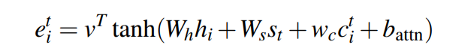
        ct = tf.expand_dims(ct, 1)score = self.V(tf.nn.tanh(  self.Wh(query) +  self.Ws(value) +  self.wc(ct)  ))attention_weights = tf.nn.softmax(score, axis=1)ct = tf.squeeze(ct,1) 
        if self.coverage is True:  
            ct+=tf.squeeze(attention_weights)context_vector = attention_weights * query
        context_vector = tf.reduce_sum(context_vector, axis=1)
 
        return context_vector, attention_weights, ct

where wc is a learnable parameter vector of the same length as v. This ensures that the attention mechanism’s current decision (choosing where to attend next) is informed by a reminder of its previous decisions (summarized in c t ). This should make it easier for the attention mechanism to avoid repeatedly attending to the same locations, and thus avoid generating repetitive text.

There is also a coverage loss to penalize repeatedly attending to the same locations.

def coverage_loss(attention_weights,coverage_vector,target): 
    mask = tf.math.logical_not(tf.math.equal(target, 0))  
    coverage_vector = tf.expand_dims(coverage_vector,axis=2)ct_min=tf.reduce_min(tf.concat
    ([attention_weights,coverage_vector],axis=2),axis=2)cov_loss = tf.reduce_sum(ct_min,axis=1)  
    mask = tf.cast(mask, dtype=cov_loss.dtype)  
    cov_loss *= mask     
    
    return cov_loss

let’s check how our summaries are generated

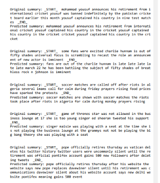
These results make a lot of sense than summaries generated by sequence to sequence and attention mechanism.

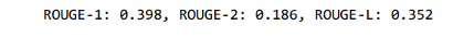
Rogue score with a seq-seq+attention+coverage mechanism

10. Pre-trained BERT

Bidirectional Encoder Representations from Transformers (BERT) advanced a wide range of natural language processing tasks. Soon after the release of the paper describing the model, the team also open-sourced the code of the model and made available for download versions of the model that were already pre-trained on massive datasets. This is a momentous development since it enables anyone building a machine learning model involving language processing to use this powerhouse as a readily-available component — saving the time, energy, knowledge, and resources that would have gone to training a language-processing model from scratch and now it can be usefully applied in text summarization for both extractive and abstractive models.

For more details about BERT check out this beautifully written blog. Here I am assuming you are familiar with BERT.

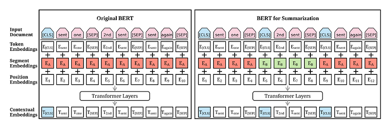
How BERT is trained for summarization

BERTSUM :

Well, we know that extractive summarization is the selection of important sentences from the document. Consider a task of implementing extractive summarization on document1 containing sentences [sent1, sent2, · · ·, sentm].

Now we can assume extractive summarization as the task of binary classification assigning a label to each sentence whether the sentence should be included in the summary or not. It is assumed that summary sentences represent the most important content of the document.

The vector for the [CLS] symbol from the top layer can be used as the representation of the sentence.

yˆi = σ(W h + bo)

Where ‘h’ is the [CLS] vector for a sentence from the top layer of the Transformer. In experiments, it is found that Transformers with L = 1, 2, 3, and found that a Transformer with L = 2 performed best. The loss of the model is the binary classification entropy of prediction yˆi against true label yi. This model is named as BERTSUM.

BERTSUMABS:

BERTSUMABS is trained for abstractive Summarization using a standard encoder-decoder framework. Here encoder is the pre-trained BERTSUM and the decoder is a 6-layered Transformer trained from scratch.

It is believable that there is a mismatch between the encoder and the decoder as the BERTSUM is pre-trained and the decoder must be trained from scratch. This can make fine-tuning uncertain. The encoder might overfit the data while the decoder under fits, or vice versa.

To avoid this, BERTSUMABS uses two separate optimizers for the encoder and the decoder.

In addition to these two strategies, there is a two-stage fine-tuning approach, where BERTSUMEXTABS first fine-tune the encoder on the extractive summarization task and then fine-tune it on the abstractive summarization task. As using extractive intentions can boost the performance of abstractive summarization.

Downloading the pretrained model on CNN daily mail data

! gdown https://drive.google.com/uc?id=1-IKVCtc4Q-BdZpjXc4s70_fRsWnjtYLr&export=download #CNN/DM Abstractive model_step_148000.pt

clone git repo

!git clone https://github.com/mingchen62/PreSumm.git

Generate summaries

!python summarizer.py -task abs -mode test  -test_from models/CNN_DailyMail_Abstractive/model_step_148000.pt \  -batch_size 6 -test_batch_size 6 -bert_data_path bert_data/cnndm \  -log_file $log_file -report_rouge False \  -sep_optim true -use_interval true \  -visible_gpus -1 -max_pos 512 \  -max_src_nsents 100 -max_length 200 \  -alpha 0.95 -min_length 50 \  -result_path $result_path \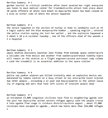

11. Fine Tuning T5

T5: TEXT-TO-TEXT-TRANSFER-TRANSFORMER

Downloading T5-small transformer from hugging face for ConditionalGeneration

tokenizer = T5Tokenizer.from_pretrained('t5-small') model = TFT5ForConditionalGeneration.from_pretrained('t5-small') task_specific_params = model.config.task_specific_params if task_specific_params is not None:     
    model.config.update(task_specific_params.get("summarization", {}))  
    
pad_token_id = tokenizer.pad_token_id

preparing data for model

def normalize_text(text):   
    text = tf.strings.lower(text)  
    text = tf.strings.regex_replace(text,"'(.*)'", r"\1")  
    return text.numpy().decode('UTF-8') def tokenize_articles(text):  
    text = normalize_text(text)  
    
    ids = tokenizer.encode_plus((model.config.prefix + text),      
    return_tensors="tf", max_length=350)
    
    return tf.squeeze(ids['input_ids']),    tf.squeeze(ids['attention_mask']) def tokenize_highlights(text):  
    text = normalize_text(text)  
    ids = tokenizer.encode(text, return_tensors="tf", max_length=50)         return tf.squeeze(ids) def map_func(x, y):      article_ids, attention_mask = tf.py_function(tokenize_articles, inp=[x], Tout=(tf.int32, tf.int32))  
    highlights_ids = tf.py_function(tokenize_highlights, inp=[y], Tout=tf.int32)      return article_ids, attention_mask, highlights_ids

Check this GitHub repo for model training

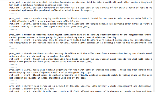
Predictions from the model:

from tqdm import tqdm 
predictions = [] 
reference=[] 
for i, (input_ids, input_mask, y) in (enumerate(test_ds)):      summaries = model.generate(input_ids=input_ids,max_length=45  ,attention_mask=input_mask)      pred = [tokenizer.decode(g, skip_special_tokens=True,   clean_up_tokenization_spaces=False) for g in summaries]      real = [tokenizer.decode(g, skip_special_tokens=True,  clean_up_tokenization_spaces=False) for g in y]       predictions.append(pred)      reference.append(real)

Generated summary

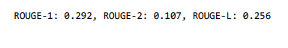
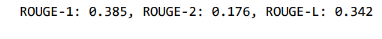
Rogue_score

12. Model Analysis

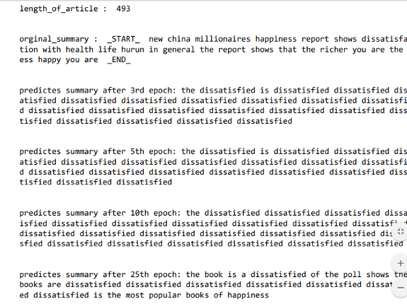
Coverage model analysis with epochs:

Let’s check how coverage vector and its loss stopped the repetition of words in prediction. Here I am printing the output of summaries after 3,5,10,25th epochs

print('length_of_article : ',len(x_train[12].split( ))) 
print('\n') print('orginal_summary : ',orgsummepoch3[12]) 
print('\n') 
print('predictes summary after 3rd epoch:',predsummepoch3[12]) print('\n') 
print('predictes summary after 5th epoch:',predsummepoch5[12]) print('\n') 
print('predictes summary after 10th epoch:',predsummepoch10[12]) print('\n') 
print('predictes summary after 25th epoch:',predsummepoch25[12])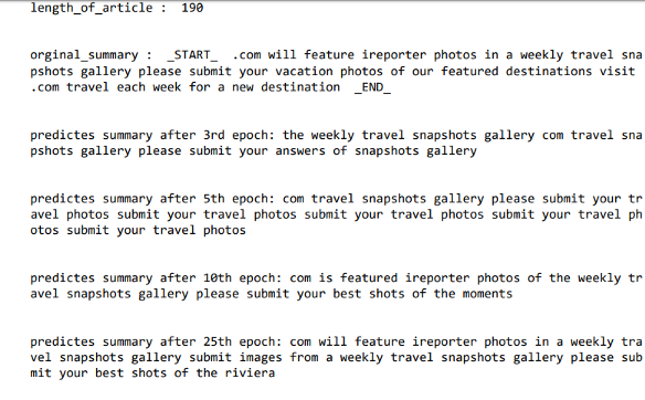

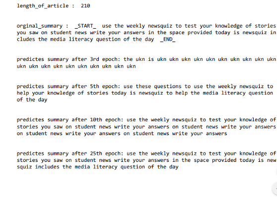
After epoch-3 generated summary is similar to output we got by attention mechanism but after epoch-10 things got changed and our coverage mechanism started and after 25th epoch, we got the precise summary

let’s analyze where our model failed

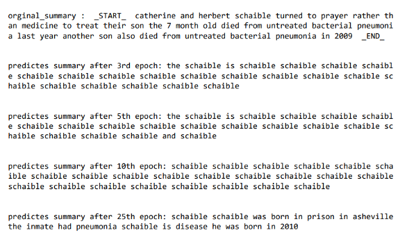
One common thing that found while analyzing the model was the length of input articles is long and some summary is meaningless. After reading the second summary from the picture it was found ridiculous…..As a predicted summary, he was born in 2010 but in org summary states he died from untreated bacterial pneumonia in 2009 which doesn’t make any sense

How good is the fine-tuned T5 model?

To check this I divided my data into 3 sets based on the article lengths

article lengths less than 200
article lengths between 200–500
article lengths more than 700

max_art_len=500 
min_art_len=200 cleaned_text = np.array(data_cleaned['text']) 
cleaned_summary = np.array(data_cleaned['summary'])
short_text = [] 
short_summary = [] 
for i in range(len(cleaned_text)):          if(len(cleaned_text[i].split())>=min_art_len and
        len(cleaned_text[i].split())<=max_art_len)        short_text.append(cleaned_text[i])        
 
        short_summary.append(cleaned_summary[i]) data1=pd.DataFrame({'text':short_text,'summary':short_summary})