Understand TensorFlow by mimicking its API from scratch

TensorFlow is a very powerful and open source library for implementing and deploying large-scale machine learning models. This makes it perfect for research and production. Over the years it has become one of the most popular libraries for deep learning.

The goal of this post is to build an intuition and understanding for how deep learning libraries work under the hood, specifically TensorFlow. To achieve this goal, we will mimic its API and implement its core building blocks from scratch. This has the neat little side effect that, by the end of this post, you will be able to use TensorFlow with confidence, because you’ll have a deep conceptual understanding of the inner workings. You will also gain further understanding of things like variables, tensors, sessions or operations.

So let’s get started, shall we?

Note: If you are familiar with the basics of TensorFlow including how computational graphs work, you may skip the theory and jump straight to the implementation part.

Theory

TensorFlow is a framework composed of two core building blocks — a library for defining computational graphs and a runtime for executing such graphs on a variety of different hardware. A computational graph has many advantages but more on that in just a moment.

Now the question you might ask yourself is, what exactly is a computational graph?

Computational Graphs

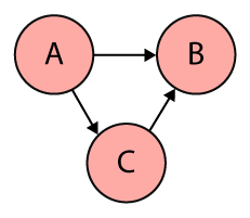
In a nutshell, a computational graph is an abstract way of describing computations as a directed graph. A directed graph is a data structure consisting of nodes (vertices) and edges. It’s a set of vertices connected pairwise by directed edges.

Here’s a very simple example:

Graphs come in many shapes and sizes and are used to solve many real-life problems, such as representing networks including telephone networks, circuit networks, road networks, and even social networks. They are also commonly used in computer science to describe dependencies, for scheduling or within compilers to represent straight line code (a sequence of statements without loops and conditional branches). Using a graph for the latter allows the compiler to efficiently eliminate common subexpression.

And of course they are used to grill people in coding interviews 😈.

Now that we have a basic understanding of directed graphs, let’s come back to computational graphs.

TensorFlow uses directed graphs internally to represent computations, and they call this data flow graphs (or computational graphs).

While nodes in a directed graph can be anything, nodes in a computational graph mostly represent operations, variables, or placeholders.

Operations create or manipulate data according to specific rules. In TensorFlow those rules are called Ops, short for operations. Variables on the other hand represent shared, persistent state that can be manipulated by running Ops on those variables.

The edges correspond to data, or multidimensional arrays (so-called Tensors) that flow through the different operations. In other words, edges carry information from one node to another. The output of one operation (one node) becomes the input to another operation and the edge connecting the two nodes carry the value.

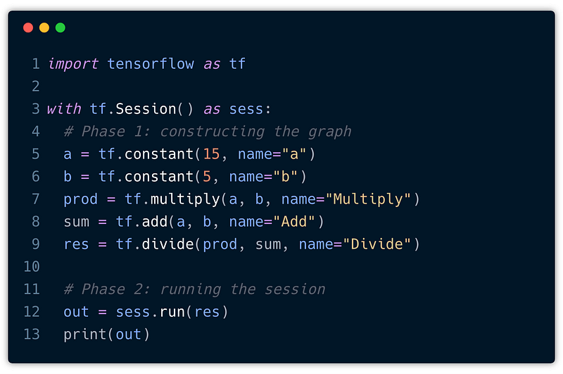
Here’s an example of a very simple program:

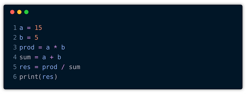
To create a computational graph out of this program, we create nodes for each of the operations in our program, along with the input variables a and b. In fact, a and b could be constants if they don’t change. If one node is used as the input to another operation we draw a directed arrow that goes from one node to another.

The computational graph for this program might look like this:

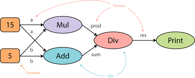
This graph is drawn from left to right but you may also find graphs that are drawn from top to bottom or vice versa. The reason why I chose the former is simply because I find it more readable.

The computational graph above represents distinct computational steps that we need to execute to arrive at our final outcome. First, we create two constants a and b . Then, we multiply them, take their sum and use the results of those two operations to divide one by the other. And finally, we print out the result.

This is not too difficult, but the question is why do we need a computational graph for this? What are the advantages of organizing computations as a directed graph?

First of all, a computational graph is a more abstract way of describing a computer program and its computations. At the most fundamental level, most computer programs are mainly composed of two things — primitive operations and an order in which these operations are executed, often sequentially, line by line. This means we would first multiply a and b and only when this expression was evaluated we would take their sum. So, the program specifies the order of execution, but computational graphs exclusively specify the dependencies across the operations. In other words, how would the output of these operations flow from one operation to another.

This allows for parallelism or dependency driving scheduling. If we look at our computational graph we see that we could execute the multiplication and addition in parallel. That’s because these two operations do not depend on each other. So we can use the topology of the graph to drive the scheduling of operations and execute them in the most efficient manner, e.g. using multiple GPUs on a single machine or even distribute the execution across multiple machines 🤯. TensorFlow does exactly this, it can assign the operations that do not depend on each other to different cores with minimal input from the person who actually writes the program, just by constructing a directed graph. That’s awesome, don’t you think?

Another key advantage is portability. The graph is a language-independent representation of our code. So we can build the graph in Python, save the model (TensorFlow uses protocol buffers), and restore the model in a different language, say C++, if you want to go really fast.

Now that we have a solid foundation let’s look at the core parts that constitute a computational graph in TensorFlow. These are the parts that we will later on re-implement from scratch.

TensorFlow Basics

A computational graph in TensorFlow consists of several parts:

• Variables: Think of TensorFlow variables like normal variables in our computer programs. A variable can be modified at any point in time, but the difference is that they have to be initialized before running the graph in a session. They represent changeable parameters within the graph. A good example for variables would be the weights or biases in a neural network.
• Placeholders: A placeholder allows us to feed data into the graph from outside and unlike variables they don’t need to be initialized. Placeholders simply define the shape and the data type. We can think of placeholders as empty nodes in the graph where the value is provided later on. They are typically used for feeding in inputs and labels.
• Constants: Parameters that cannot be changed.
• Operations: Operations represent nodes in the graph that perform computations on Tensors.
• Graph: A graph is like a central hub that connects all the variables, placeholders, constants to operations.
• Session: A session creates a runtime in which operations are executed and Tensors are evaluated. It also allocates memory and holds the values of intermediate results and variables.

Remember from the beginning that we said TensorFlow is composed of two parts, a library for defining computational graphs and a runtime for executing these graphs? That’s the Graph and Session. The Graph class is used to construct the computational graph and the Session is used to execute and evaluate all or a subset of nodes. The main advantage of deferred execution is that during the definition of the computational graph we can construct very complex expressions without directly evaluating them and allocating the space in memory that is needed.

For example, if we use NumPy to define a large matrix, say a trillion by a trillion, we would immediately get an out of memory error. In TensorFlow we would define a Tensor that is a description of a multidimensional array. It may have a shape and a data type but it does not have an actual value.

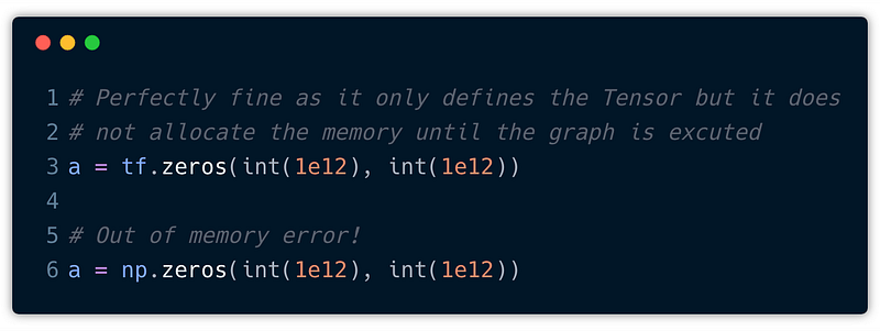
In the snippet above we use both tf.zeros and np.zeros to create a matrix with all elements set to zero. While NumPy will immediately instantiate the amount of memory that is needed for a trillion by a trillion matrix filled with zeros, TensorFlow will only declare the shape and the data type but not allocate the memory until this part of the graph is executed. Cool, right?

This core distinction between declaration and execution is very important to keep in mind, because this is what allows TensorFlow to distribute the computational load across different devices (CPUs, GPUs, TPUs) attached to different machines.

With those core building blocks in place, let’s convert our simple program into a TensorFlow program. In general, this can be divided into two phases:

1. Construction of the computational graph.
2. Running a session

Here’s what our simple program could look like in TensorFlow:

We start off by importing tensorflow. Next, we create a Session object within a with statement. This has the advantage that the session is automatically closed after the block was executed and we don’t have to call sess.close() ourselves. Also, these with blocks are very commonly used.

Now, inside the with-block, we can start constructing new TensorFlow operations (nodes) and thereby define the edges (Tensors). For example:

a = tf.constant(15, name="a")

This creates a new Constant Tensor with the name a that produces the value15. The name is optional but useful when you want to look at the generated graph, as we’ll see in just a moment.

But the question now is, where is our graph? I mean, we haven’t created a graph yet but we are already adding these operations. That’s because TensorFlow provides a default graph for the current thread that is an implicit argument to all API functions in the same context. In general, it’s enough to rely solely on the default graph. However, for advanced use cases we can also create multiple graphs.

Ok, now we can create another constant for b and also define our basic arithmetic operations, such as multiply, add, and divide. All of these operations are added automatically to the default graph.

That’s it! We completed the first step and constructed our computational graph. Now it’s time to compute the result. Remember, until now nothing has been evaluated and no actual numeric values have been assigned to any of those Tensors. What we have to do is to run the session to explicitly tell TensorFlow to execute the graph.

Ok, this one is easy. We already created a session object and all we have to do is to call sess.run(res) and pass along an operation (here res) that want to evaluate. This will only run as much of the computational graph as needed to compute the value for res. This means that in order to compute res we have to compute prod and sum as well as a and b. Finally, we can print the result, that is the Tensor returned by run().

Cool! Let’s export the graph and visualize it with TensorBoard:

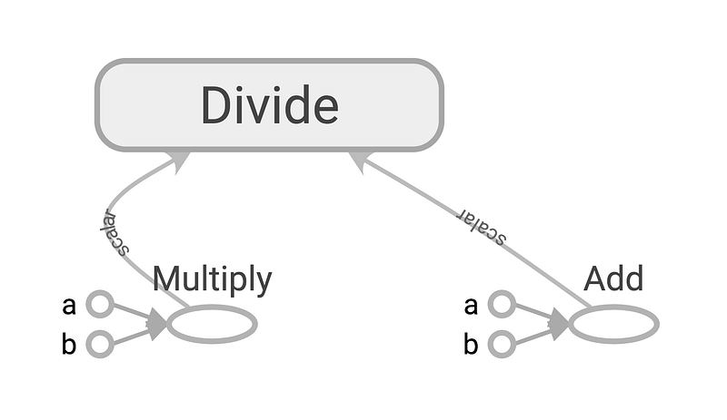
This looks very familiar, doesn’t it?

By the way, TensorBoard is not only great for visualizing learning but also to look and debug your computational graphs, so definitely check it out.

Ok, enough theory! Let’s get straight into coding.

Implementing TensorFlow’s API from scratch

Our goal here is to mimic the basic operations from TensorFlow in order to mirror our simple program with our own API, just like we did a moment ago with TensorFlow.

Earlier, we learned about some of the core building block, such as Variable, Operation, or Graph. These are the building blocks we want to implement from scratch, so let’s get started.

Graph

The first missing piece is the graph. A Graph contains a set of Operation objects, which represent units of computation. In addition, a graph contains a set of Placeholder and Variable objects, which represent the units of data that flow between operations.

For our implementation we essentially need three lists to store all those objects. Furthermore, our graph needs a method called as_default which we can call to create a global variable that is used to store the current graph instance. This way, we don’t have to pass around the reference to the graph when creating operations, placeholders or variables.

So, here we go:

Operations

The next missing piece are operations. To recall, operations are the nodes in the computational graph and perform computations on Tensors. Most operations take zero or many Tensors as input, and produce zero or more Tensors objects as output.

In a nutshell, an operation is characterized as follows:

1. it has a list of input_nodes
2. implements a forward function
3. implements a backward function
4. remembers its output
5. adds itself to the default graph

So, each node is only aware of its immediate surrounding, meaning it knows about its local inputs coming in and its output that is directly being passed on to the next node that is consuming it.

The input nodes is a list of Tensors (≥ 0) that are going into this operation.

Both forward and backward are only placeholder methods and they must be implemented by every specific operation. In our implementation, forward is called during the forward pass (or forward-propagation) which computes the output of the operation, whereas backward is called during the backward pass (or backpropagation) where we calculate the gradient of the operation with respect to each input variable. This is not exactly how TensorFlow does it but I found it easier to reason about if an operation it fully autonomous, meaning it knows how to compute an output and the local gradients with respect to each of the input variables.

Note that in this post we will only implement the forward pass and we’ll look at the backward pass in another post. This means we can just leave the backward function empty and don’t worry about it for now.

It’s also important that every operation is registered at the default graph. This comes in handy when you want to work with multiple graphs.

Let’s take one step at a time and implement the base class first:

We can use this base class to implement all kinds of operations. But it turns out that the operations we are going to implement in just a moment are all operations with exactly two parameters a and b. To make our life a little bit easier and to avoid unnecessary code duplication, let’s create a BinaryOperation that just takes care of initializing a and b as input nodes.

Now, we can use the BinaryOperation and implement a few more specific operations, such as add, multiply, divide or matmul(for multiplying two matrices). For all operations we assume that the inputs are either simple scalars or NumPy arrays. This makes implementing our operations simple, because NumPy has already implemented them for us, especially more complex operations such as the dot product between two matrices. The latter allows us to easily evaluate the graph over one batch of samples and compute an output for each observation in the batch.

Placeholder

When we look at our simple program and its computational graph, we can notice that not all nodes are operations, especially a and b. Rather, they are inputs to the graph that have to be supplied when we want to compute the output of the graph in a session.

In TensorFlow there are different ways for providing input values to the graph, such as Placeholder, Variable or Constant. We have already briefly talked about each of those and now it’s time to actually implement the first one — Placeholder.

As we can see, the implementation for a Placeholder is really simple. It’s not being initialized with a value, hence the name, and only appends itself to the default graph. The value for the placeholder is provided using the feed_dict optional argument to Session.run(), but more on this when we implement the Session.

Constant

The next building block we are going to implement are constants. Constants are quite the opposite of variables as they cannot be changed once initialized. Variables on the other hand, represent changeable parameters in our computational graph. For example, the weights and biases in a neural network.

It definitely makes sense to use placeholders for the inputs and labels rather than variables, as they always change per iteration. Also, the distinction is very important as variables are being optimized during the backward pass while constants and placeholders are not. So we cannot just simply use a variable for feeding in constant. A placeholder would work, but that also feels a bit misused. To provide such feature, we introduce constants.

In the above we are leveraging a feature from Python in order to make our class a little bit more constant like.

Underscores in Python have a specific meaning. Some are really just convention and others are enforced by the Python interpreter. With the single underscore _ most of it is by convention. So if we have a variable called _foo then this is generally seen as a hint that a name is to be treated as private by the developer. But this isn’t really anything that is enforced by the interpreter, that is, Python does’t have these strong distinctions between private and public variables.

But then there is the double underscore __ or also called “dunder”. The dunder is treated differently by the interpreter and it’s more than just a convention. It actually applies naming mangling. Looking at our implementation we can see that we are defining a property __value inside the class constructor. Because of the double underscore in the property name, Python will rename the property internally to something like _Constant__value, so it prefixes the property with the class name. This feature is actually meant to prevent naming collisions when working with inheritance. However, we can make use of this behavior in combination with a getter to create somewhat private properties.

What we did is we created a dunder property __value, exposed the value through another “publicly” available property value and raise a ValueError when someone tries to set the value. This way, users of our API cannot simply reassign the value unless they would invest a little bit more work and find out that we are using a dunder internally. So it’s not really a true constant and more like const in JavaScript, but for our purpose it’s totally ok. This at least protects the value from being easily reassigned.

Variable

There is a qualitative difference between inputs to the computational graph and “internal” parameters that are being tuned and optimized. As an example, take a simple perceptron that computes y = w * x + b. While x represents the input data, w and b are trainable parameters, that is, variables within the computational graph. Without variables training a neural network wouldn’t be possible. In TensorFlow, variables maintain state in the graph across calls to Session.run() unlike placeholders that must be provided with every call to run().

Implementing variables is easy. They require an initial value and append themselves to the default graph. That’s it.

Session

At this point, I’d say we feel quite confident constructing computational graphs and we have implemented the most important building blocks to mirror TensorFlow’s API and rewrite our simple program with our own API. There’s just one last missing piece that we have to build — and that’s the Session.

So, we have to start thinking about how to compute the output of an operation. If we recall from the beginning, this is exactly what the session does. It’s a runtime in which operations are executed and the nodes in our graph are evaluated.

From TensorFlow we know that a session has a run method, and of course several other methods but we are only interested in this particular one.

At the end, we want to be able to use our session as follows:

session = Session()
output = session.run(some_operation, {
    X: train_X # [1,2,...,n_features]
})

So run takes two parameters, an operation to be executed and a dictionary feed_dict that maps graph elements to values. This dictionary is used to feed in values for the placeholders in our graph. The operation that is provided is a graph element that we want to compute an output for.

In order to compute an output for the given operation, we have to topologically sort all nodes in the graph to make sure we execute them in the correct order. This means that we cannot evaluate Add before we evaluate our constants a and b.

Topological ordering can be defined as an ordering of the nodes in a directed acyclic graph (DAG) where for each directed edge from node A to node B, node B appears before A in the ordering.

The algorithm is pretty straight forward:

1. Pick any unvisited node. In our example, this is the last computational node in the graph which is passed to Session.run().
2. Perform depth-first search (DFS) by recursively iterating over the input_nodes of each node.
3. If we reach a node that has no more inputs, mark that node as visited and add it to the topological ordering.

Here’s an animated illustration of the algorithm in action for our specific computational graph:

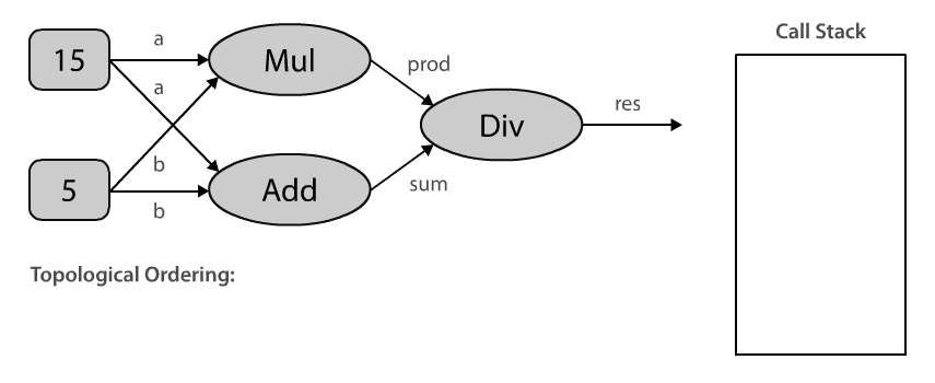
When we topologically sort our computational graph beginning with Div, we end up with an ordering where the constants are evaluated first, then the operations Mul and Add , and finally Div. Note that topological orderings are not unique. The ordering could also be 5, 15, Add, Mul, Div, and it really depends on the order in which we process the input_nodes. This makes sense, doesn’t it?

Let’s create a tiny utility method topologically sorts a computational graph starting from a given node.

Now that we can sort a computational graph and make sure the nodes are in the correct order, we can start working on the actual Session class. This means creating the class and implementing the run method.

What we have to do is the following:

1. topologically sort the graph beginning from the operation provided
2. iterate over all nodes
3. differentiate between different types of nodes and compute their output.

Following these steps, we end up with an implementation that could like this:

It’s important that we differentiate between the different types of nodes because the output for each node may be computed in a different way. Remember that, when executing the session we only have actual values for variables and constants but placeholders are still waiting for their value. So when we compute the output for a Placeholder we have to look up the value in the feed_dict provided as a parameter. For variables and constants we can simply use their value as their output, and for operations we have to collect the output for each input_node and call forward on the operation.

Wohoo 🎉! We did it. At least we have implemented all the parts needed to mirror our simple TensorFlow program. Let’s see if it actually works, shall we?

For that, let’s put all the code for our API in a separate module called tf_api.py. We can now import this module and start using what we have implemented.

When we run this code, assuming we have done everything right so far, it will correctly print out 3.75 to the console. This is exactly what we wanted to see as an output.

This looks intriguingly similar to what we did with TensorFlow, right? The only difference here is the capitalization, but that was on purpose. While in TensorFlow literally everything is an operation — even placeholders and variables — we didn’t implement them as operations. In order to tell them apart, I have decided to lowercase operations and capitalize the rest.

Try it out for yourself in this Repl!

Conclusion

Congratulations 👏, you have successfully implemented some core APIs from TensorFlow. Along the way we have discovered computational graphs, talked about topological ordering and managed to mirror a simple TensorFlow program using our own API. By now I hope that you feel confident enough to start using TensorFlow, if you haven’t already.

While writing this post, I was diving deep into the source code of TensorFlow and I am really impressed by how well written the library is. With that said, I want to emphasize once more that what we have implemented is not 100% how things work in TensorFlow, because there are quite some abstractions and TensorFlow is way more complete, but I wanted to make things easier and reduce it to the core concepts.

I hope that this post was helpful for you and that TensorFlow is now a little less intimidating.

Where to go next?

In this post we have implemented the foundation and in another post, we’ll build on top of this and implement the backward pass including a Gradient Descent optimizer. This will be fore sure another fun journey. Till then, happy coding! 🙌

Oh and if you have any remarks, feel free to leave a comment below or reach out to me on Twitter!

Special Thanks

I’d like to thank William Horton, Matthijs Hollemans and Kwinten Pisman for reviewing the article and providing valuable feedback. 🙏