
Ultimate Guide to Statistics for Data Science
Statistics at a glance for data science: standard guidelines
Motivation
Statistics is a powerful mathematical field. I’m saying “powerful” because it helps us to infer a population outcome from sample data. As it can infer population outcome, it can also be used for the big picture (like overall impact, future forecast, etc.). Statistics is not just a combination of some merely isolated topics. Moreover, Statistics discovers new semantics within these topics, which sometimes paves the way for new opportunities. Statistics needs everywhere in our day-to-day life. The main problem I faced in my junior year was that I couldn’t relate statistical knowledge to real life. I was unknown where to use which techniques to find the answer and act accordingly. The new journey began when I started to learn data science back in 2018. I covered all the basic statistics topics needed for data science and realized how necessary the knowledge of statistics is! As a lecturer of Artificial Intelligence and Data Science at a University, I conduct statistics classes and try to represent it as a useful tool for our regular usage. I also want to share the knowledge throughout my write-ups. That’s why I have written a series of articles covering all the basic topics of statistics and tried to represent them in the easiest possible way. Though some topics are missed in the series, I will try to integrate them into this article along with my previous works. I hope every walk of people will easily understand these articles on statistics. No prerequisite is required. Finally, I want to say, “this article covers most (but not all!) topics, and it will provide a base of statistics for data science so that you can explore other advanced topics if needed.”
So, if you are an absolute beginner to statistics and searching for a complete guideline, this article is gonna be for you.
Table of Contents
The next section is the most important part of this article where all the articles in this series will be linked with brief descriptions.
Topic Description with Embedded Links
Statistics at a Glance
As per my understanding, statistics combines some techniques for drawing a reliable conclusion about a large group (population) by experimenting on a small group (sample) and summarizing the dataset. It is not a formal definition; it’s my realization while working with statistics.
Let’s look at a formal definition according to Wikipedia [1] -
Statistics is the discipline that concerns the collection, organization, analysis, interpretation, and presentation of data.
There are two categories of statistics.
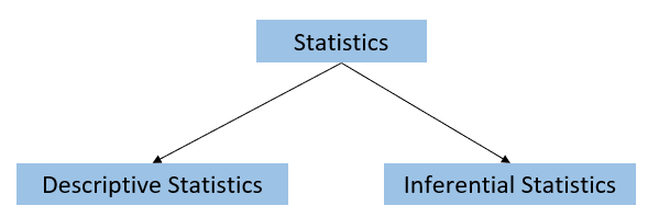
- Descriptive statistics summarizes/describes the population or sample dataset. It covers the topics —
types of data, variables, data representation, frequency distribution, central tendency, percentile and quartile, covariance, correlation, etc. - Inferential statistics is part of statistics that finds reliable inferences of population data from sample data. It covers —
probability distribution, Central Limit Theorem, Point Estimator and Estimate, Standard Error, Confidence Interval and Level, Level of Significance, Hypothesis Testing, Analysis of Variance (ANOVA), Chi-Square Test, etc.
Population and Sample
The population consists of all the members of an experiment, whereas sample is a selected group of members from the population which represents that population.
For example, we want to know university students’ average CGPA. Here, the experimental area covers all the students. So, the population will be all the students of that university. If we pick some students to calculate the average CGPA, these students will be the sample.
Before jumping to statistics, you must clearly understand the topics.
To make your idea crystal clear please read the following article —
Variable and Level of Measurement
Simply variable is something which can vary (hold multiple values). It is nothing but the features of a dataset. There are different types of data as different features exist in the real world. We must know the measurement level to understand how we deal with the data.
If you have any confusion about the topic, go through the article.
Central Tendency
Central tendency is a way to find out the tendency of majority values. In statistics, mean, median, and mode are used to know it.
- Mean
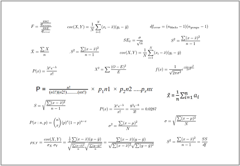
The concept of “mean” is straightforward. We get the mean value by dividing the summation by the number of values (n).

Complete Mean Guideline —
- Median
The Median is another way to know the central tendency. To get the median value, we need to sort the values in ascending order and pick up the middle value, it varies with the even and odd number of values.
For example, 12, 13, 10, 15, and 7 are the series of values. Firstly, we need to sort out the values. After sorting, the sequence will be 7, 10, 12, 13, and 15. The total number of values is 5, which is an odd number. So, we will use the following formula —

In our case, 12 is the median.
Another example is that some values are 12, 13, 10, 15, 7, and 9. After sorting, we get 7, 9, 10, 12, 13, and 15. This time, the number of values is 6, and it’s even. So, we won’t get the middle value with the above formula. Because (6+1)/2= 3.5 is not a whole number. Now, we need to sum up the 3rd and 4th values. And their mean is the median value, 22/2 = 11.
Python Implementation —
- Mode
The mode works on categorical data, and it is the highest frequency of a dataset. Suppose you have some data containing the quality of a product like [‘good’, ‘bad’, ‘normal’, ‘good’, ‘good’]. Here, good has the highest frequency. So, it is the mode for our data.
Python Implementation —
When to use which central tendency?
In the case of nominal data, we use mode. For ordinal data, the median is recommended. Mean is widely used to find the central tendency of ratioed / interval variables. But the mean is not always the right choice to determine the central tendency because if the dataset contains outliers, the mean will be very high or low. In that case, the median is more robust than the mean. We will use the median if the median is greater or less than the mean. Otherwise, mean is the best choice.
For more details, click here.
Percentile, Quartile and IQR
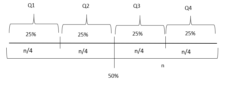
- Percentile
A percentile is a measure used in statistics indicating the value below which a given percentage of observations in a group of observations fall. For example, the 20th percentile is the value (or score) below which 20% of the observations may be found [2].
- Quartile
In the percentile, the entire values are divided into 100 different parts. The quartile divides the values into four equal parts, and each part holds 25%. The main quartiles are First Quartile (Q1), Second Quartile (Q2), Third Quartile (Q3) and Fourth Quartile (Q4).
- IQR (Inter Quartile Ratio)
IQR is the range between Q1 and Q3. So, IQR = Q1 — Q3 .
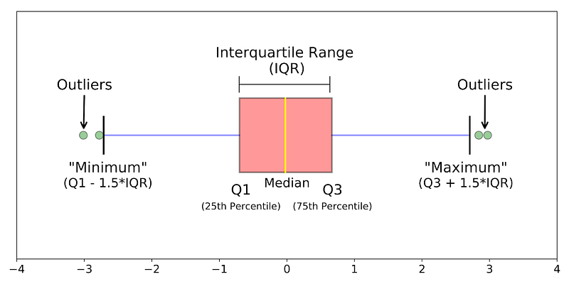
We can also find out the outlier with IQR by defining a minimum (Q1 -1.5*IQR, also known as lower fence) and maximum (Q3 + 1.5*IQR, also known as upper fence) boundary value. Outside the minimum and maximum values are considered outliers.
Boxplot shows all the Quartiles and upper and lower fences.
Frequency Distribution and Visualization
Frequency is the measure of the occurrence of an event in a dataset. The following articles will help you to know details about the topic.
Measure of Dispersion
The concept Measure of Dispersion indicates how spread the values are! Range, Variance, Standard Deviation. etc., are some of the techniques to find dispersion.
- Range
The range is the interval of maximum and minimum values. For example, we have some sample data 12, 14, 20, 40, 99, and 100. The range will be (100–12) = 88.
- Variance
Variance measures the difference between each value of a dataset from the mean value. According to Investopedia —
Variance measures how far each number in the set is from the mean (average), and thus from every other number in the set [5].

Here, x̄ is the sample mean and n is the number of values.

μ is the population mean and N is the number of population values.
- Standard Deviation
Standard Deviation is the square root of variance.


Python implementation of variance and standard deviation —
Covariance and Correlation
- Covariance
Covariance is a way to compare the variance between two numerical variables. The following formula is used to calculate it.

Here, x and y represent two variables. N is the number of the population.
- Correlation (Pearson Correlation)
It finds the linear relationship between two numerical variables.

The correlation value fluctuates between -1 to +1. -1 indicates an entirely negative relationship, whereas +1 indicates a completely positive relationship between the variables. And 0 means no relationship.
Python Implementation —
Normalization
Normalization is the process of converting the data into similar scale and it is one of the key parts of data pre-processing. The following article integrates all the techniques for data normalization.
Probability
Probability is a mathematical technique by which we can predict the probable outcome of an event. Read the following articles if you have any confusion about probability.
Probability Distribution
The probability distribution is the distribution of all the probabilities of an event. There are two types of the probability distribution.
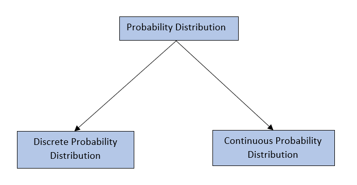
- Discrete Probability Distribution
The discrete probability distribution is the probability distribution of discrete values. For example, the probability of rolling a die. We find a specific outcome for each role, and it’s obvious a discrete value.
Uniform distribution, Binominal distribution, Poisson distribution, etc., are some of the main discrete probability distributions.
- Continuous Probability Distribution
The continuous probability distribution is the probability distribution of continuous value. For example, the probability of being age 24 of a sample group. As age 24 is a continuous value, we need to use continuous probability distribution.
Normal distribution, Student’s t distribution, etc., are some of the continuous probability distributions.
- Discrete Uniform Distribution
In uniform distribution, all the values of specific outcomes are equal. For example, rolling dice has 6 individual outcomes = {1,2,3,4,5,6}. If it is uniformly distributed, each probability value is 0.16667.
Python Implementation [6] —
- Binomial Distribution
The name “Binomial” suggests two mutually exclusive outcomes of trials. For instance, head or tail, good or bad, pass or fail, etc.
For Binominal distribution, a trial must satisfy the criteria of the Bernoulli Trial.
The Bernoulli trial must have two independent outcomes like, high or low. The probability of success must be constant.

Here, n is the number of trials, p is the probability of success, and the number of successes x.
Let’s plot a binominal distribution for rolling dice. Suppose you roll a die 16 times. What will be the probability that 2 comes up 4 times? Here, p=1/6 and n=16. The binominal distribution for the scenario is shown with python code.
[The article [7] helps me to implement the code.]
The red bar indicates the probability of 2, comes up 4 times.
- Poisson distribution
The red bar indicates the probability of 2, which comes up 4 times.
- Poisson distribution
Binomial distribution finds the number of successes out of a specific number of trials. Poisson distribution determines the number of successes within a unit of time interval.
For example, in a shop 8 customers arrive between 12 pm to 1 pm. With the help of Poisson distribution, we can find out the probability of arriving 3 people between 12 pm to 1 pm. Poisson distribution can be explained with the following formula.

Where x is the number of successes, λ is the number of occurrences per unit of time. ε is the Euler number (2.71828…). For the above problem, x=3, λ=8/1=8.

Red bar shows the probability of arriving 3 customers between 12pm to 1pm.
- Normal Distribution
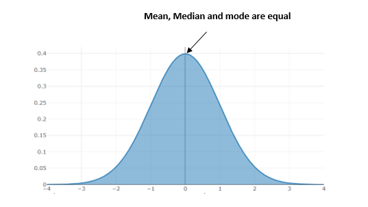
The continuous probability distribution is applicable to continuous variables. The normal distribution is one of the widely used continuous probability distributions. Many real-life problems can be solved/described with normal distribution. Suppose we consider a sample age of 70 students. The age ranges from 18 to 25 years. It will be normally distributed if the mean, mode, and median are equal in that sample.
In case of normal distribution, the probability of the left and right parts being equally distributed means it is symmetrical. Total probability equal to 1. The distribution follows the following equation.

Here, σ is the standard deviation and μ is the mean.
Normal distribution with python —
Normal distribution will be a standard normal distribution when the standard deviation is 1, and the mean value is 0. Below is an example of the standard normal distribution with python.
- Student’s t distribution
William Sealy Gossett proposed the distribution. As there is a restriction in his working place to publish research articles with the original name, he used his pseudonym, “Student.” The distribution was proposed to find out the best sample from a small sample [8].
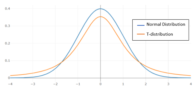
The image shows the comparison of two distributions. Student’s T-distribution has a fatter a tail than the normal distribution. Python implementation of student’s t distribution [9].
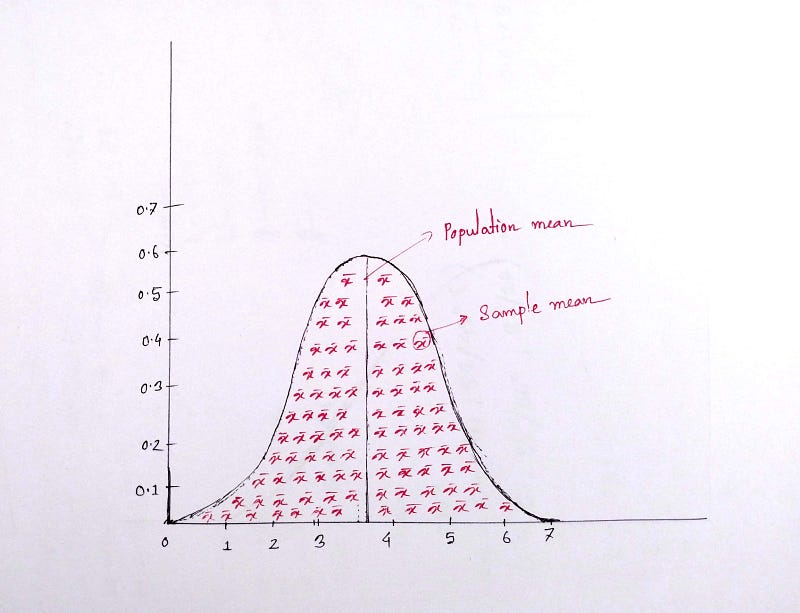
Central Limit Theorem
If we randomly make huge samples from a population and consider the mean values, we will find that sample values will be normally distributed around the population mean. It’s a way to find out good sample data.
Estimator and Estimate
Estimators are the terms of statistics by which we estimate some facts about the population [10]. Some estimators are the sample mean, standard deviation, variance, etc.
The value of the estimator is known as the estimate.
Suppose the variance of a sample is 5. Here, the variance is the estimator, and the value of the variance is called the estimate.
Standard Error
Standard deviation indicates how far the values are from the population mean, and standard error shows how far sample means are from the population mean. It is calculated as follows —

Here, σ is the population standard deviation, and n is the sample size.
Confidence Level and Interval
- Confidence Level
The confidence level is the percentage value; within that value the parameter’s truth value will remain. Suppose we have solved a problem with a 95% confidence level; that means 95% time, we will get the accurate result from our solved problem.
- Confidence interval
The confidence interval is a range within which we will get the truth value of the confidence level.
Significance Level
The significance level of an event (such as a statistical test) is the probability that the event could have occurred by chance. If the level is quite low, that is, the probability of occurring by chance is quite small, we say the event is significant [11].
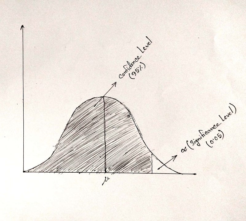
Significance level is denoted by α symbol.
Hypothesis Testing
Hypothesis testing is a statistical technique by which we can test and validate an assumption. In hypothesis testing, we consider a null hypothesis, which is assumed to be true, and an alternative hypothesis, which is acceptable if the null hypothesis fails. More details about Hypothesis testing is given in the following article.
Analysis of Variance (ANOVA)
In the Hypothesis testing article, I have mentioned some tests like p-test, t-test, etc., but those tests only compare between two groups. None of them can be used for multiple groups. ANOVA is a statistical test used for comparing the variability between two or more groups. Detail explanation has been provided in the article below.
Chi-Square Test
The Chi-Square test is another statistical test for finding the dependency of categorical variables. Go through the following article.
Conclusion
Statistics is an integral part of data science. Each and every topic of statistics can’t be covered because the field is huge. However, I have tried to cover the important knowledge of statistics needed for data science. With this article, I am going to wrap up my series writing on statistics for data science. If you have any questions, feel free to inform me in the comment section.
Thank You
References
- Statistics — Wikipedia
- Percentile. IAHPC Pallipedia. https://pallipedia.org/percentile/. Accessed October 16, 2022.
- All the Basics of Frequency Distribution | Towards Data Science
- https://towardsdatascience.com/compare-multiple-frequency-distributions-to-extract-valuable-information-from-a-dataset-10cba801f07b
- What Is Variance in Statistics? Definition, Formula, and Example (investopedia.com)
- https://pyshark.com/continuous-and-discrete-uniform-distribution-in-python/
- Python — Binomial Distribution — GeeksforGeeks
- Dunnett, C. W., & Sobel, M. (1954). A bivariate generalization of Student’s t-distribution, with tables for certain special cases. Biometrika, 41(1–2), 153–169.
- Python — Student’s t Distribution in Statistics — GeeksforGeeks
- Estimator: Simple Definition and Examples — Statistics How To
- https://www.sciencedirect.com/topics/mathematics/significance-level-alpha


