Summary

The website content provides an overview of various groundbreaking Convolutional Neural Network (CNN) architectures, including LeNet-5, AlexNet, VGG-16 Net, ResNet, and Inception Net, detailing their unique features, contributions, and drawbacks.

Abstract

The article discusses the evolution of CNN architectures in the field of computer vision, starting with LeNet-5, which was designed for character recognition. It then delves into AlexNet, which introduced deeper architectures and won the ImageNet ILSVRC-2012 competition. The VGG-16 Net is highlighted for simplifying the architecture by using multiple 3x3 filters and for its significant number of parameters. ResNet is noted for its deep networks with skip connections and batch normalization, which helped to train networks with over 100 layers. Finally, the Inception Net, or GoogleLe Net, is described for its innovative use of parallel filters of different sizes to capture features at various scales, and its subsequent versions aimed to reduce computational cost while maintaining accuracy.

Opinions

LeNet-5 is recognized as a classic and straightforward neural network for handwritten digit recognition.
AlexNet is acknowledged for its depth and the introduction of new techniques such as ReLU, data augmentation, and dropout, but it is also criticized for having too many hyper-parameters.
VGG-16 Net is praised for its simplicity and effectiveness but is critiqued for its long training time, heavy model size, computational expense, and susceptibility to vanishing/exploding gradient problems.
ResNet is celebrated for enabling the training of very deep networks without degradation in performance, thanks to skip connections and batch normalization.
Inception Net is admired for its novel approach to feature extraction using parallel pathways with different kernel sizes, although the original version was computationally intensive, leading to the development of more efficient versions like Inception v2 and v3.

Types of Convolutional Neural Networks: LeNet, AlexNet, VGG-16 Net, ResNet and Inception Net

We would be seeing different kinds of Convolutional Neural Networks and how they differ from each other in this article. These are some groundbreaking CNN architectures that were proposed to achieve a better accuracy and to reduce the computational cost .

1. LeNet-5

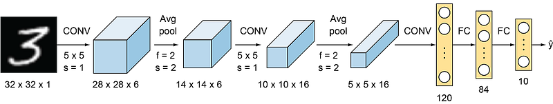
This is also known as the Classic Neural Network that was designed by Yann LeCun, Leon Bottou, Yosuha Bengio and Patrick Haffner for handwritten and machine-printed character recognition in 1990’s which they called LeNet-5. The architecture was designed to identify handwritten digits in the MNIST data-set. The architecture is pretty straightforward and simple to understand. The input images were gray scale with dimension of 32*32*1 followed by two pairs of Convolution layer with stride 2 and Average pooling layer with stride 1. Finally, fully connected layers with Softmax activation in the output layer. Traditionally, this network had 60,000 parameters in total. Refer to the original paper.

2. AlexNet

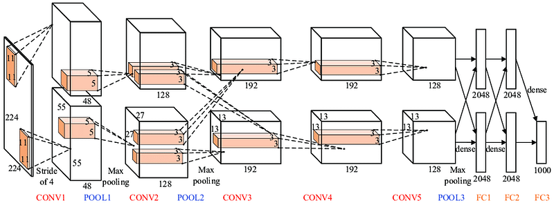
This network was very similar to LeNet-5 but was deeper with 8 layers, with more filters, stacked convolutional layers, max pooling, dropout, data augmentation, ReLU and SGD. AlexNet was the winner of the ImageNet ILSVRC-2012 competition, designed by Alex Krizhevsky, Ilya Sutskever and Geoffery E. Hinton. It was trained on two Nvidia Geforce GTX 580 GPUs, therefore, the network was split into two pipelines. AlexNet has 5 Convolution layers and 3 fully connected layers. AlexNet consists of approximately 60 M parameters. A major drawback of this network was that it comprises of too many hyper-parameters. A new concept of Local Response Normalization was also introduced in the paper. Refer to the original paper.

3. VGG-16 Net

The major shortcoming of too many hyper-parameters of AlexNet was solved by VGG Net by replacing large kernel-sized filters (11 and 5 in the first and second convolution layer, respectively) with multiple 3×3 kernel-sized filters one after another. The architecture developed by Simonyan and Zisserman was the 1st runner up of the Visual Recognition Challenge of 2014. The architecture consist of 3*3 Convolutional filters, 2*2 Max Pooling layer with a stride of 1, keeping the padding same to preserve the dimension. In total, there are 16 layers in the network where the input image is RGB format with dimension of 224*224*3, followed by 5 pairs of Convolution(filters: 64, 128, 256,512,512) and Max Pooling. The output of these layers is fed into three fully connected layers and a softmax function in the output layer. In total there are 138 Million parameters in VGG Net.

Drawbacks of VGG Net: 1. Long training time 2. Heavy model 3. Computationally expensive 4. Vanishing/exploding gradient problem

4. ResNet

ResNet, the winner of ILSVRC-2015 competition are deep networks of over 100 layers. Residual networks are similar to VGG nets however with a sequential approach they also use “Skip connections” and “batch normalization” that helps to train deep layers without hampering the performance. After VGG Nets, as CNNs were going deep, it was becoming hard to train them because of vanishing gradients problem that makes the derivate infinitely small. Therefore, the overall performance saturates or even degrades. The idea of skips connection came from highway network where gated shortcut connections were used.

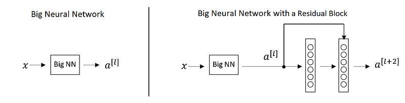
Normal Deep Networks vs Networks with skip connections

For the above figure for network with skip connection, a[l+2]=g(w[l+2]a[l+1]+ a[l])

Lets say for some reason, due to weight decay w[l+2] becomes 0, therefore, a[l+2]=g(a[l])

Hence, the layer that is introduced doesnot hurt the performance of the neural network. This the reason, increasing layers doesn’t decrease the training accuracy as some layers may make the result worse. The concept of skip connections can also be seen in LSTMs.

5. Inception Net

Inception network also known as GoogleLe Net was proposed by developers at google in “Going Deeper with Convolutions” in 2014. The motivation of InceptionNet comes from the presence of sparse features Salient parts in the image that can have a large variation in size. Due to this, the selection of right kernel size becomes extremely difficult as big kernels are selected for global features and small kernels when the features are locally located. The InceptionNets resolves this by stacking multiple kernels at the same level. Typically it uses 5*5, 3*3 and 1*1 filters in one go. For better understanding refer to the image below:

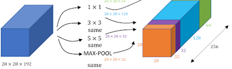
Note: Same padding is used to preserve the dimension of the image.

As we can see in the image, three different filters are applied in the same level and the output is combined and fed to the next layer. The combination increases the overall number of channels in the output. The problem with this structure was the number of parameter (120M approx.) that increases the computational cost. Therefore, 1*1 filters were used before feeding the image directly to these filters that act as a bottleneck and reduces the number of channels. Using 1*1 filters, the parameter were reduced to 1/10 of the actual. GoogLeNet has 9 such inception modules stacked linearly. It is 22 layers deep (27, including the pooling layers). It uses global average pooling at the end of the last inception module. Inception v2 and v3 were also mentioned in the same paper that further increased the accuracy and decreasing computational cost.

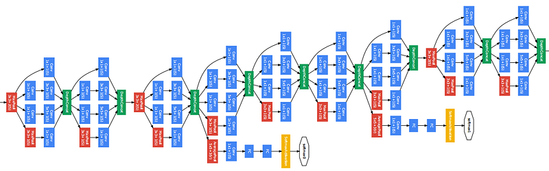
Several Inception modules are linked to form a dense network

Side branches can be seen in the network which predicts output in order to check the shallow network performance at lower levels.