Data Science

Two Interesting Pandas Data Manipulation Functions You Need to Know

Extremely useful pandas functions for converting a continuous pandas column into categorical ones.

Python pandas is a powerful and widely used library for data analysis.

It comes up with 200+ functions and methods, making data manipulation and transformation easy. However, knowing all these functions and using them where required in the actual work isn’t a feasible task.

One of the common tasks in data manipulation is converting a column having continuous numerical values into a column containing discrete or categorical values. And pandas has two amazing built-in functions which can certainly save you a few minutes.

You can use such type of data transformation for a variety of applications like grouping data, analyzing data by discrete groups, or visualizing data using histograms.

For example,

Recently, I calculated Herfindahl-Hirschman Index (HHI) to understand the market concentration of multiple brands. So in a pandas DataFrame, I had a column with continuous values of HHI for all brands. Ultimately, I wanted to convert this column to a discrete one to categorize each brand as low, medium, and high market concentration — That’s where I got inspired for this story.

Without knowing these built-in pandas functions, you might need to write multiple if-else and for statements to get the same work done.

Therefore, here you’ll explore such 2 super-useful built-in pandas functions along with interesting examples (including my project), which will supercharge your data analysis and save you a couple of minutes.

Often you need to convert a column with continuous values into another column with discrete values in your analytics project.

So basically you categorize the continuous data into several categories, i.e. buckets or bins. And you can do so by either specifying minimum and maximum values for each bin, i.e. defining bin edges or by specifying the number of bins.

Depending on your purpose of splitting a continuous series into a discrete one, you can use one of the next two methods.

As I was curious about a built-in function for my work, first I came across the cut() function from pandas library.

pandas cut()

You can use pandas cut() when you want to split the data into a fixed number of different buckets, irrespective of the number of values in each bucket.

As per pandas official documentation, there are 7 optional parameters for the function pandas.cut() along with 2 mandatory parameters.

But you don’t need to remember all of them.

I’ve simplified things for you. I’m using this function quite often nowadays and found some of the function parameters more useful than others.

Here are the commonly used optional parameters which you’ll use in almost 90% of the cases.

pandas.cut(x,
           bins,
           labels=None,
           right=True,
           include_lowest=False)

Let’s take an example to understand how each of these parameters works.

Suppose you have the following continuous series, which you would like to convert into 5 bins.

import pandas as pd
import numpy as np

# Create random data
Series1 = pd.Series(np.random.randint(0, 100, 10))

# Create DataFrame
df = pd.DataFrame({"Series1": Series1})

# Apply pandas.cut() on the column Series1
df["binned_Series1"] = pd.cut(df["Series1"], bins=5)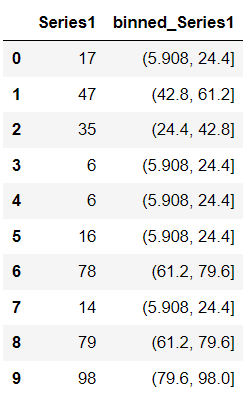

You simply assigned the integer 5 to the parameter bin — as a result, pandas split the entire column Series1 into 5 equal-sized buckets. Pandas assigned each value from Series1 to one of these 5 buckets.

If you inspect each of these buckets, you’ll see two things are common.

1. The bin edges are non-integer — You can fix this by defining the bin edges in the bin parameter.
2. Each bin edge is closed on the right — It is coming from the default setting of the parameter right as right=True. It means that the pandas include the maximum value of the bucket in the same bucket. This parameter specifically helps you control the binning process and switching its value helps you include or exclude certain elements from a bin.

Let’s give it a second chance.

This time you’ll pass a list of bin edges for the same DataFrame column and see how the result changes.

df["binned_Series1_defined_binedge"] = pd.cut(df["Series1"],
                                              bins=[0, 10, 15, 40, 65, 100])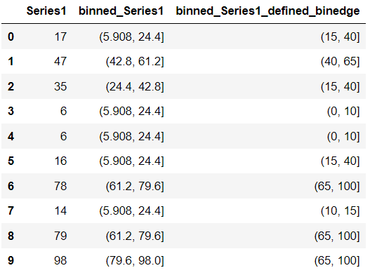

Pandas simply created new bins using the integers you provided in the bin parameter and assigned each number of Series1 to these bins.

Moreover, you can also use the Label parameter to give a name to each of these buckets, like below.

df["bin_name"] = pd.cut(df["Series1"],
                        bins=[0, 10, 15, 40, 65, 100],
                        labels=['bin 1', 'bin 2', 'bin 3', 'bin 4', 'bin 5'])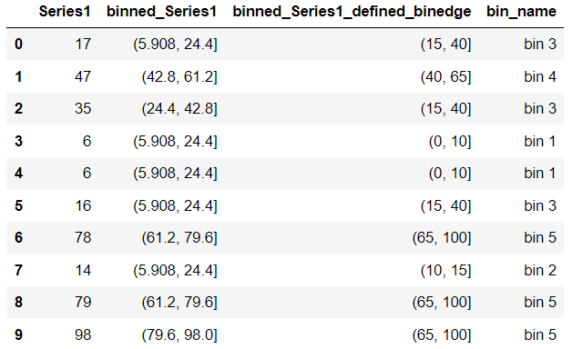

It works perfectly as expected!

Coming back to my work — a real-world scenario — I tried the function pandas.cut() on my below dataset.

# Create a sample DataFrame as I can not disclose the original data
HHI = [random.random() for i in range(10)]
Brands = ["Brand_1", "Brand_2", "Brand_3", "Brand_4", "Brand_5",
          "Brand_6", "Brand_7", "Brand_8", "Brand_9", "Brand_10"]

df = pd.DataFrame({"brand": Brands, "hhi": HHI})

# Use pandas.cut()
df["binned_hhi"] = pd.cut(df["hhi"], bins=3)
df["brand_bucket"] = pd.cut(df["hhi"], 
                            bins=3, 
                            labels = ["low", "medium", "high"])
df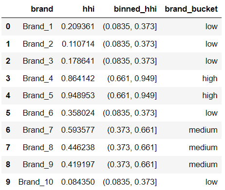

However, the distribution of elements in each of these buckets is uneven, i.e. each bin contains a different number of elements. 5 brands belong to the low, 3 brands belong to the medium, and only 2 brands belong to the high concentration bucket.

But for my project, I wanted to keep the distribution i.e. the number of brands in each bucket same and that’s where I found the next pandas method useful.

pandas qcut()

pandas.qcut() is used to get an equal data distribution in all the bins. It works on the principle of sample quantiles.

Quantiles are the values that divide a series into a number of subsets — each containing nearly the same number of elements.

So when you cut a series using the function qcut(), it simply tells you which element`of the series belongs to which quantile.

The basic syntax of the function qcut() is almost the same as the syntax of the function cut().

Let’s understand this with an example — Here you’ll use both the functions cut() and qcut() on the same data and categorize them into 4 bins.

Series1 = pd.Series([17, 47, 35, 6, 6, 16, 78, 14, 79, 98])
df = pd.DataFrame({"Series1": Series1})

df["qcut_Series1"] = pd.qcut(df["Series1"], q=4) # Use qcut()
df["cut_Series1"] = pd.cut(df["Series1"], bins=4) # Use cut()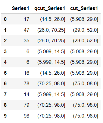

Now, when you check the data distribution in each bin —

# Check the data distribution of each bucket when cut() was used
df["cut_Series1"].value_counts()

#Output
(5.908, 29.0]    5
(75.0, 98.0]     3
(29.0, 52.0]     2
(52.0, 75.0]     0
Name: cut_Series1, dtype: int64


# Check the data distribution of each bucket when qcut() was used
df["qcut_Series1"].value_counts()

#Output
(5.999, 14.5]    3
(70.25, 98.0]    3
(14.5, 26.0]     2
(26.0, 70.25]    2
Name: qcut_Series1, dtype: int64

You’ll see when you used the function cut(), although each bin size is equal, i.e. 23, each bin contains a different number of elements.

Whereas, when you used the function qcut(), a similar number of elements were present in each bucket. But you can see such distribution came at the cost of varied bin sizes.

So in the case of my project, the function pandas.qcut() was the ultimate solution as you can see here —

df["binned_hhi_qcut"] = pd.qcut(df["hhi"], q=3)
df["brand_bucket_qcut"] = pd.qcut(df["hhi"], 
                            q=3, 
                            labels = ["low", "medium", "high"])
df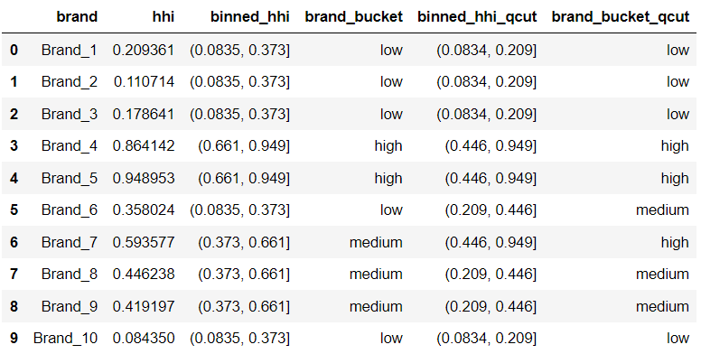

So, qcut() assigned 3 brands to each of the medium and high concentration buckets and 4 brands to the low concentration bucket.

I hope you found this article refreshing and useful. Although the conversion of a continuous series into discrete ones is the common scenario in data analysis, the task can be really daunting if you don’t know the built-in functions.

Using these functions in your data analysis projects will certainly empower you to easily extract the required information from the data in no time.

LMK in the Comments which topics you would like to get such amazing articles!

Well, just knowing these functions is not enough — start using them in your data analysis tasks to unlock the real pandas power today.

Ready to level up your data analysis skills?

💡 Consider Becoming a Medium Member to access unlimited stories on Medium and daily interesting Medium digest. I will get a small portion of your fee and No additional cost to you.

💡 Be sure to Sign-up to my Email list to never miss another article on data science guides, tricks, and tips, SQL, and Python.

To know more about my project, Comment your question!

Thank you for reading!