Tune Deep Neural Networks using Bayesian Optimization

Leverage Bayesian Theory to boost your performance

In a previous post, we presented a case study about Image Classification using Tensorflow and Deep Learning Methods.

Although the case study was minimal, it showcased every stage of a machine learning project: Cleaning, preprocessing, model building, training, and evaluation. But we skipped tuning.

In this article, we will delve a little deeper into hyperparameter optimization. Again, we will use the Fashion MNIST[1] dataset, which is included in Tensorflow.

As a reminder, the dataset contains 60,000 grayscale images in the training set and 10,000 images in the test set. Each image represents a fashion item that belongs to one of 10 categories (‘T-shirt/top’, ‘Trouser’, ‘Pullover’, and so on). Hence, we have a multi-class classification problem.

I’ve launched AI Horizon Forecast, a newsletter focusing on time-series and innovative AI research. Subscribe here to broaden your horizons!

Setup

I will go over briefly the steps for preparing the dataset. For more information, check the first part of the previous article: In short, the steps are:

Load the data.
Split into training, validation, and test sets.
Normalize pixel values from 0–255 to 0–1 range.
One-hot encode the target variable.

To recap, the shapes of all training, validation, and test sets are:

Hyperparameter tuning

Now, we will use the Keras Tuner library [2]: It will help us tune the hyperparameters of our neural networks with ease. To install it, execute:

pip install keras-tuner

Note: Keras Tuner requires Python 3.6+ and TensorFlow 2.0+

As a quick reminder, hyperparameter tuning is a fundamental part of a machine learning project. There are two types of hyperparameters:

Structural hyperparameters: Those define the overall architecture of a model (e.g. number of hidden units, number of layers)
Optimizer hyperparameters: Those influence the speed and the quality of training (e.g. learning rate and type of optimizer, batch size, number of epochs)

Why tuning is tricky?

Why the need for a hyperparameter tuning library? Can’t we just try every possible combination and see what’s best on the validation set?

Unfortunately, no:

Deep neural networks take a lot of time to train, even days.
If you train large models on the cloud (like Amazon Sagemaker), remember that each experiment costs money.

Therefore, a pruning strategy that limits the search space of hyperparameters is necessary.

Bayesian optimization

Luckily, Keras tuner provides a Bayesian Optimization tuner. Instead of searching every possible combination, the Bayesian Optimization tuner follows an iterative process, where it chooses the first few at random. Then, based on the performance of those hyperparameters, the Bayesian tuner selects the next best possible.

Thus, each choice of hyperparameters depends on the previous attempts. The number of iterations for choosing the next set of hyperparameters based on history and evaluating performance continues until the tuner finds the best combination or exhausts the maximum number of trials. We can configure this with the argument ‘max_trials’.

The Keras tuner provides two more tuners: RandomSearch and Hyperband, apart from the Bayesian Optimization tuner. We will talk about them at the end of this article.

Back to our Example

Next, we are going to apply hyperparameter tuning to our networks. In the previous article, we experimented with two network architectures, the standard Multilayered Perceptron (MLP) and the Convolutional Neural network (CNN).

Multilayered Perceptron (MLP)

But first, let’s remember what our baseline MLP model was:

The tuning process requires two main methods:

hp.Int(): Sets the range of hyperparameters whose values are integer - for example, the number of hidden units in a Dense layer:

model.add(Dense(units = hp.Int('dense-bot', min_value=50, max_value=350, step=50))

2. hp.Choice(): Provides a set of values for a hyperparameter — for example, Adam or SGD as the best optimizer?

hp_optimizer=hp.Choice('Optimizer', values=['Adam', 'SGD'])

Hence, using the Bayesian Optimization tuner on our original MLP example, we test the following hyperparameters:

Number of Hidden layers: 1–3
First Dense Layer size: 50–350
Second and third Dense Layer size: 50–350
Dropout Rate: 0, 0.1, 0.2
Optimizers: SGD(nesterov=True, momentum=0.9) or Adam
Learning Rates: 0.1, 0.01, 0.001

Notice the for-loop at line 5: We let the model decide the depth of our network!

Finally, we start the tuner. Notice the max_trials argument that we mentioned previously.

This will print:

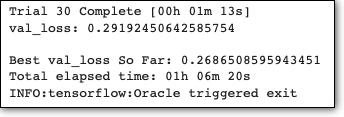
The process exhausted the number of iterations and took ~1 hour to finish. We can also print the optimal hyperparameters of our model, using the following command:

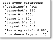
And that’s it! We can now retrain our model using the optimal hyperparameters:

Alternatively, we can retrain our model with less verbosity:

All we have to do now is check the test accuracy:

# Test accuracy: 0.8823

Compared to the baseline’s model test accuracy:

Baseline MLP model: 86.6 % Best MLP model: 88.2 %

Indeed, we observe a difference of ~3% in test accuracy!

Convolutional Neural networks (CNNs)

Again, we are going to follow the same procedure. With CNNs, we have a few more parameters that we can test.

First, this was our baseline model:

The baseline model only contains a single set of filtering and pooling layers. For our tuning, we will test the following:

Number of “blocks” of Convolutional, MaxPooling, and Dropout layers
Filter size of Conv layers in each block: 32, 64
Valid or same padding on Conv Layers
Hidden layer size of a final extra layer: 25–150, by 25
Optimizers: SGD (nesterov=True, momentum=0.9) or Adam
Learning Rates: 0.01, 0.001

Like before, we let the network decide its depth.

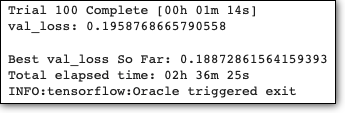
Now, we are ready to call the Bayesian Tuner. The maximum number of iterations is set to 100:

This will print:

And the best hyperparameters are:

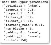
Finally, we train our CNN model using the best hyperparameters:

And check the accuracy of the test set:

# Test accuracy: 0.92

Compared to the baseline’s CNN model test accuracy (from our previous article):

Baseline CNN model: 90.8 % Best CNN model: 92%

Again, we saw a performance increase with the optimized model!

Apart from accuracy, we can confirm that the tuner did his job well because of the following:

The tuner chose a non-zero Dropout value in every case, even though we supplied the tuner with zero Dropout as well. That is expected, because Dropout is an invaluable mechanism that reduces overfitting.
Interestingly, the best CNN architecture is the standard pipeline where the number of filters gradually increase in each layer. This is expected, because as computations move forward in subsequent layers, the patterns gets more complex. Hence, there are more pattern combinations that require more filters in order to be captured.

Closing Remarks

Undoubtedly, Keras Tuner is a versatile tool for optimizing deep neural networks with Tensorflow.

The most obvious choice is the Bayesian Optimization tuner. However, there are two more options that someone could use:

RandomSearch: This type of tuner avoids exploring the whole search space of hyperparameters by selecting a few of them at random. However, it does not guarantee that this tuner will find the optimal ones.
Hyperband: This tuner chooses some random combinations of hyperparameters and uses them to train the model for a few epochs only. Then, the tuner uses those hyperparameters to train the model until all epochs are exhausted and chooses the best among them.

Thank you for reading!

Follow me on Linkedin!
Subscribe to my newsletter, AI Horizon Forecast!

AutoGluon-TimeSeries : Creating Powerful Ensemble Forecasts — Complete Tutorial

Amazon’s framework for time-series forecasting has it all.

aihorizonforecast.substack.com

References

Keras Tuner, https://keras.io/keras_tuner/

References

- Fashion MNIST dataset by Zalando, https://www.kaggle.com/datasets/zalando-research/fashionmnist, MIT Licence (MIT) Copyright © [2017]