Summary

The TS2Vec review discusses a novel approach for learning universal time series representations through hierarchical contrasting.

Abstract

TS2Vec introduces a method for time series representation learning that leverages hierarchical contrasting to capture both local and global dependencies within the data. It involves sampling overlapping subseries and enforcing consistency in their contextual representations, using an input projection layer to map observations into a high-dimensional space, and applying a random mask layer to improve generalization. The architecture includes a ConvEncoder composed of 1D residual convolutional blocks, and it employs both instance and temporal contrastive losses to learn discriminative representations. The learned representations are versatile for various downstream tasks, such as classification, where they can be max-pooled or encoded at multiple scales to obtain hierarchical encodings.

Opinions

The authors believe that the TS2Vec model's ability to handle raw time series data without the need for domain-specific data preprocessing is a significant advantage.
The use of a random mask layer is seen as crucial for handling the potentially unbounded value range of time series data and for preventing overfitting.
The hierarchical structure of the model, which includes both instance and temporal contrastive losses, is considered essential for capturing the complex temporal dependencies in time series data.
The model's flexibility in adapting to different downstream tasks by providing both single-scale and multi-scale representations is highlighted as a key strength.
The authors suggest that the TS2Vec approach represents a step towards universal time series representation learning, implying that it could be broadly applicable across various time series analysis domains.

TS2vec review: Towards universial time series representation learning with hierarchical contrasting

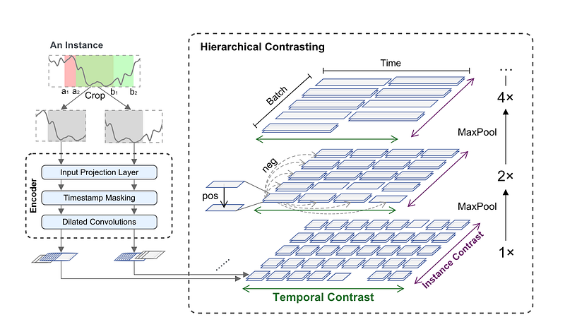
First, We randomly sample two overlapping subseries from an in-put time series xi, and encourage consistency of contextual representations on the common segment.

out1 = self._net(take_per_row(x, crop_offset + crop_eleft, crop_right - crop_eleft))
out1 = out1[:, -crop_l:]

out2 = self._net(take_per_row(x, crop_offset + crop_left, crop_eright - crop_left))
out2 = out2[:, :crop_l]

Second, for the TS2Vec encoder

Input Projection layer: For each input xi, the input projec-tion layer is a fully connected layer that maps the observation into a high dimensional space ( set to be 64) by default. This was implemented as a linear layer.

B x T x input_dims is transformed into B x T x Ch. I believe this handles multi-variate time series and projects them into the hidden space. Note that we mask latent vectors rather than raw values because the value range for time series is possibly unbounded and it is impossible to find a special token for raw data.

The random mask layer: This is applied across each sample and timepoint, similar to drop out wheras we are setting randomly selected timepoints to be 0. The default mask is a binomial mask equilvent to a coin flip.

def generate_binomial_mask(B, T, p=0.5):
    return torch.from_numpy(np.random.binomial(1, p, size=(B, T))).to(torch.bool)

The ConvEncoder is made up of a sequence of a 1D res-conv1d blocks. Each block consists of two 1d-D convolutional layer

Loss

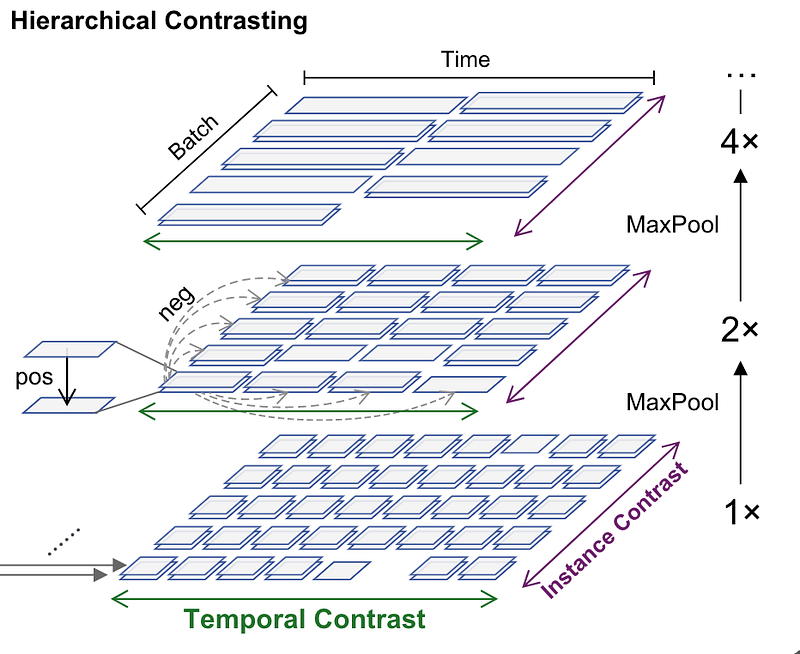
To learn discriminative representations over time, TS2Vec takes the representations at the same timestamp from two views of the input time se-ries as positives, while those at different timestamps fromthe same time series as negatives.

The input to the loss computation are the features from the previous encoder step in dimensions B x T x Co (batch_number x timestamps x outoput dimension from the last conv layer)

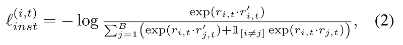
At each level, VS2Vec calculates the instance contrastive loss,

Instance Contrastive Loss where B is batch size. This is a modified version of InfoNCE loss.

"""
1. Concatenate the two sets of embeddings (z1, z2) into a single tensor (z).
2. Compute the similarity matrix between all pairs of embeddings (sim).
3. Compute the logits (logits) for the similarity matrix (sim).
   The logits are the log-probabilities of the similarity matrix
   conditioned on the fact that the embeddings are from the same
   sequence or from different sequences.
4. Compute the loss by taking the mean over all pairs of embeddings
   of the log-probability of the similarity matrix conditioned on
   the fact that the embeddings are from the same sequence or from
   different sequences. 
"""

def instance_contrastive_loss(z1, z2):
    B, T = z1.size(0), z1.size(1)
    if B == 1:
        return z1.new_tensor(0.)
    z = torch.cat([z1, z2], dim=0)  # 2B x T x C
    z = z.transpose(0, 1)  # T x 2B x C
    sim = torch.matmul(z, z.transpose(1, 2))  # T x 2B x 2B
    logits = torch.tril(sim, diagonal=-1)[:, :, :-1]    # T x 2B x (2B-1)
    logits += torch.triu(sim, diagonal=1)[:, :, 1:]
    logits = -F.log_softmax(logits, dim=-1)
    
    i = torch.arange(B, device=z1.device)
    loss = (logits[:, i, B + i - 1].mean() + logits[:, B + i, i].mean()) / 2
    return loss

The temporal contrastive loss is as follows, which is highly similar to the implementation above. Notice that the similarity computation is done across T (timestamps), not across 2B (augmented data batch pairs).

def temporal_contrastive_loss(z1, z2):
    B, T = z1.size(0), z1.size(1)
    if T == 1:
        return z1.new_tensor(0.)
    z = torch.cat([z1, z2], dim=1)  # B x 2T x C
    sim = torch.matmul(z, z.transpose(1, 2))  # B x 2T x 2T
    logits = torch.tril(sim, diagonal=-1)[:, :, :-1]    # B x 2T x (2T-1)
    logits += torch.triu(sim, diagonal=1)[:, :, 1:]
    logits = -F.log_softmax(logits, dim=-1)
    
    t = torch.arange(T, device=z1.device)
    loss = (logits[:, t, T + t - 1].mean() + logits[:, T + t, t].mean()) / 2
    return loss

The above loss compute is recursively computed and added, meaning that we start from the timestamps level to compute the terms, , apply max_pool kernel (default 2) which increases receptive field by 2 and re-compute the loss terms until we cannot divide by time dimension any more.

Applying to downstream task

We apply SGD to learn the encoder with the self-supervised setup above to a given dataset.

For classification tasks, the classes are labeled on the entiretime series (instance). Therefore we require the instance-level representations, which can be obtained by max pool-ing over all timestamps, meaning that hidden value representation would be reduced to single maximal value per timepoint. Alternatively, you can specificy an encoding window or set to multiscale encoding to recusively obtain the encoding at each level before maxpool 1d, yielding a Hierarchical encoding of multiple scales.