Neural Networks

Transposed Convolutional Neural Networks — How to Increase the Resolution of Your Image

A Detailed Explanation of Transposed Convolutions with a Simple Python Example

Intro

Convolutional Neural Networks revolutionized the space of image categorization and object detection. But have you heard about Transposed Convolutions, and would you know how to use them?

In this article, I will explain what Transposed Convolutions are, how they compare to regular Convolutions and show you how to build a simple Neural Network that utilizes them for image resolution upscaling.

Contents

• Transposed Convolutions within the universe of Machine Learning algorithms
• What is Transposed Convolution?
• What are Transposed Convolutions used for?
• A complete Python example of building a Neural Network with Transposed Convolutions in Keras/Tensorflow

Transposed Convolutions within the universe of Machine Learning algorithms

I have categorized Machine Learning algorithms based on their nature and the job they are designed to do. You can see this categorization in the chart below.

While it is impossible to do this perfectly since some algorithms can be assigned to multiple categories, an attempt to bring some structure enables us to visualize how these different algorithms connect and compare.

The chart is interactive, so you can explore it by clicking👇 on different categories to reveal more. Unsurprisingly, you will find Transposed Convolutional Networks under the Convolutional Neural Network branch.

If you enjoy Data Science and Machine Learning, please subscribe to get an email with my new articles. If you are not a Medium member, you can join here.

What is Transposed Convolution?

Note, in some literature, Transposed Convolutions are also referred to as Deconvolutions or Franctionally Strided Convolutions.

To understand Transposed Convolutions, let’s first remind ourselves what a regular Convolution is.

Convolution

There are three parts to a convolution: an input (e.g., 2D image), a filter (a.k.a. kernel) and an output (a.k.a. convolved feature).

The convolution process is iterative. First, a filter is applied over a section of an input image, and the output value is recorded. The filter is then shifted by one position when stride=1 or by multiple positions when the stride is set to a higher number, and the same process is repeated until the convolved feature is complete.

The below gif image illustrates the process of applying a 3x3 filter on a 5x5 input.

Transposed Convolution

The goal of a Transposed Convolution is to do the opposite of a regular Convolution, i.e., to upsample the input feature map to a desired larger size output feature map.

To achieve this, Transposed Convolution goes through an iterative process of multiplying entries in the input feature map by the filter and adding them up together. Note that we also move along by the specified number of places (stride) within each step.

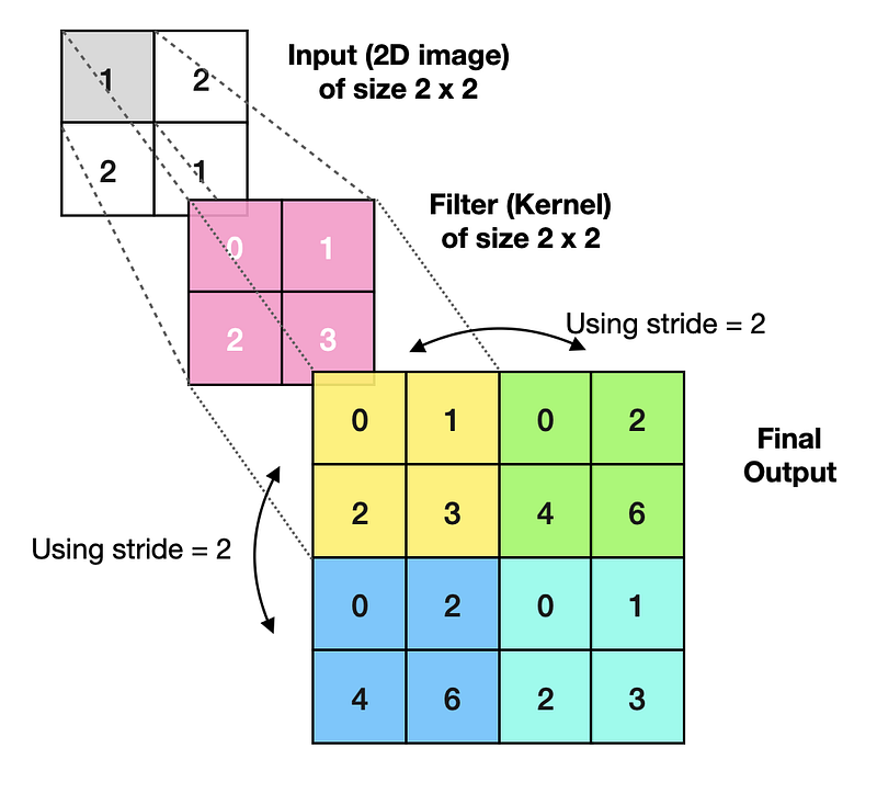
The below gif illustrates how the Transposed Convolution works. The example moves from a 2x2 input to a 3x3 output via a 2x2 filter using a stride of 1.

• Take the first input entry and multiply it by the filter matrix. Temporarily store the result.
• Then, take the second input entry and multiply it by the filter matrix. Temporarily store the result. Continue this process for the rest of the input matrix.
• Finally, sum up all the partial outputs to get the final result.

It is worth noting that we are essentially generating additional data during the transposed convolution operation as we are upsampling the feature map from a smaller to a larger size.

However, this operation is not exactly the reverse of a Convolution. It is because some information is always lost during a Convolution, meaning that we can never precisely recreate the same data by applying a Transposed Convolution.

Lastly, we can experiment with a filter size or stride to achieve the desired size of an output feature map. E.g., we could increase the stride from 1 to 2 to avoid section overlaps and produce a 4x4 output (see image below).

What are Transposed Convolutions used for?

Transposed Convolutions are crucial for Semantic Segmentation and data generation in the Generative Adversarial Networks (GANs). One of the more straightforward examples would be a Neural Network trained to increase image resolution. We will build one such network right now.

A complete Python example that utilizes Keras/Tensorflow

Setup

We will need to get the following data and libraries:

• Caltech 101 image data set (source)

Data license: Attribution 4.0 International (CC BY 4.0)

Reference: Li, F.-F., Andreeto, M., Ranzato, M. A., & Perona, P. (2022). Caltech 101 (Version 1.0) [Data set]. CaltechDATA. https://doi.org/10.22002/D1.20086

• Pandas and Numpy for data manipulation
• Open-CV, Matplotlib and Graphviz for ingesting and displaying images and showing a model diagram
• Tensorflow/Keras for building Neural Networks
• Scikit-learn library for splitting the data (train_test_split)

Let’s import the libraries:

The above code prints package versions that I used in this example:

Tensorflow/Keras: 2.7.0
pandas: 1.3.4
numpy: 1.21.4
sklearn: 1.0.1
OpenCV: 4.5.5
matplotlib: 3.5.1
graphviz: 0.19.1

Next, we download, save and ingest Caltech 101 image data set. Note that I will only use images of pandas (Category = “panda”) in this example instead of an entire list of 101 categories.

At the same time, I prep the data and save images in two different resolutions:

• 64 x 64 pixels, which will be our low-res input data.
• 256 x 256 pixels, which will be our hi-res target data.

The above code prints the shape of our data, which is [samples, rows, columns, channels].

Shape of whole data_lowres:  (38, 64, 64, 3)
Shape of whole data_hires:  (38, 256, 256, 3)
Shape of X_train:  (30, 64, 64, 3)
Shape of Y_train:  (30, 256, 256, 3)
Shape of X_test:  (8, 64, 64, 3)
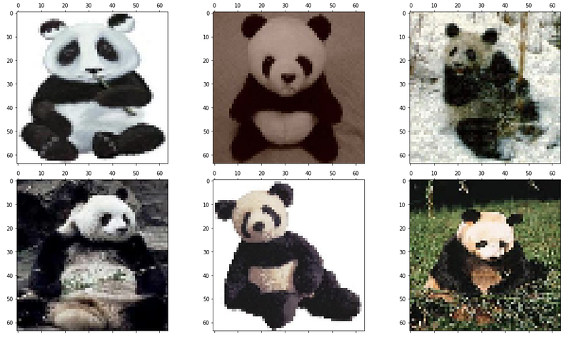
Shape of Y_test:  (8, 256, 256, 3)

To better understand what data we are working with, let’s display a few low-res images that we will use as inputs.

And a few hi-res images to be used as targets in our model.

Training and evaluating Transposed Convolutional Neural Network

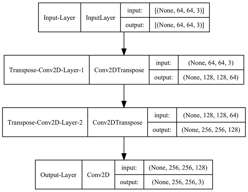
This model is very simple, containing an Input layer, two Transposed Convolutional layers, and a final Convolutional layer that acts as Output. You can follow comments in the code to understand what each section does.

Here is the model diagram:

Next, I train the model over 100 epochs.

Once training is complete, we can use the model to predict (upscale) low-res images to a higher resolution. Let’s look at a couple of examples, one from the training set and another from the test set.

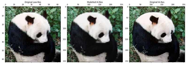
Display an image comparison from a training set:

Display an image comparison from a test set:

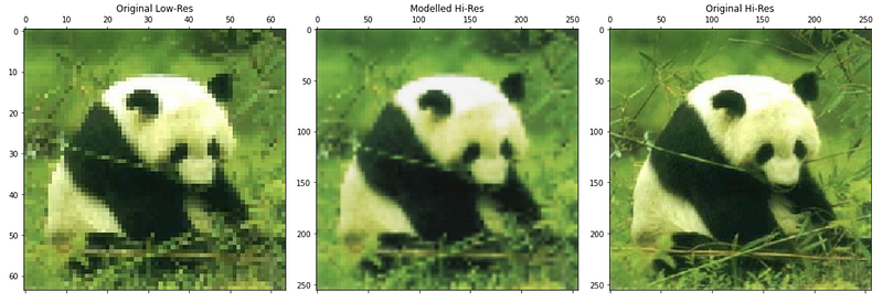
We can see that we were able to increase image resolution somewhat successfully in both examples above. I.e., the individual pixels are less apparent in the modelled image.

However, we did lose some sharpness, which is noticeable when compared to our target (256 x 256) image. One can experiment with model parameters to achieve better results as my model is by no means optimised.

Final remarks

I sincerely hope you enjoyed reading this article and gained some new knowledge.

You can find a complete Jupyter Notebook code in my GitHub repository. Feel free to use it to build your own Transposed Convolutional Neural Networks, and do not hesitate to get in touch if you have any questions or suggestions.

You can subscribe here if you would like to be notified when I publish a new article, e.g., on Semantic Segmentation or GANs.

Also, feel free to check out my other Neural Network articles: Feed-Forward, Deep Feed-Forward, CNN, RNN, LSTM, GRU, AE, DAE, SAE, and VAE.

Cheers! Saul Dobilas