Summary

The web content discusses various methods of data transformation, including normalization and scaling, to prepare raw data for better analysis and model creation by achieving a more Gaussian distribution and equalizing feature scales.

Abstract

Raw data often comes in distributions that are not conducive to analysis or model creation, necessitating preprocessing transformations. The goal of these transformations is to normalize data into a Gaussian distribution, which typically yields better model results due to the balance of observations around the mean. Normalization adjusts data to a common scale without altering the range, while scaling changes the data range, often to fit within a specific interval. Common methods for data transformation include log transformation to reduce skewness, min-max scaling to a fixed range, standardization to a mean of 0 and standard deviation of 1, unit vector transformation to adjust vector length without changing direction, mean normalization to distribute features between [-1, 1], and Box Cox transformation to stabilize variance and normalize dependent variables. These techniques are crucial for machine learning algorithms, ensuring that data is appropriately shaped for optimal analysis.

Opinions

Normalization is particularly useful when the data distribution is known to be non-Gaussian.
Scaling is essential for comparing variables on an equal basis, especially in distance-based models where variable magnitude can introduce bias.
Log transformation is highly effective for addressing skewed data and facilitating inferential statistics.
Min-Max scaling, while useful for fitting data into a specific range, can suppress the influence of outliers.
Standardization is preferred over normalization when outliers are significant and should not be discarded.
Unit vector transformation maintains the integrity of vector direction while adjusting its magnitude.
Mean normalization is a method that centers the data around zero with a standard deviation of one.
Box Cox transformation is recommended for positive data to achieve normality and stabilize variance, with the caveat that all data points must be positive.

Transformations, Scaling and Normalization

By: Isabella Lindgren

Raw data comes in all kinds of strange distributions so sometimes it is difficult to analyze and especially to create models without some preprocessing. There are a variety of ways to shape the data into a more favorable input, so here is a quick break down of a few commonly used methods of transforming our data!

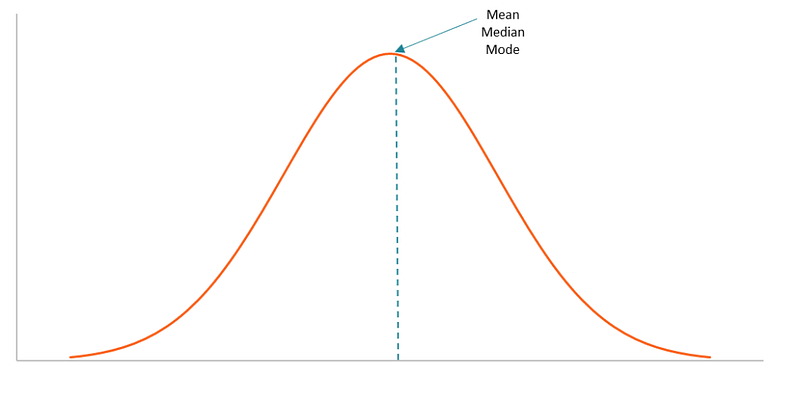
The overall goal of transforming our data is to create a more normal (*Gaussian*) distribution aka a bell curve. In general, normal distributions tend to produce better results in a model because there are about equal observations above and below the mean and the mean and median are the same. Models run under the assumption your data is normally distributed.

By transforming our data we are not only normalizing the observations, but the residuals as well. Normalization makes training models less sensitive to the scale of features, so we can better solve for coefficients. The coefficients are statistical measures of the degree in which the changes to the value of one variable predict change to the value of another variable. Normalizing and scaling are two types of transformations that are important in data cleaning.

So what is the difference between Normalizing and Scaling?

The main difference between normalizing and scaling is that in normalization you are changing the shape of the distribution and in scaling you are changing the range of your data. Normalizing is a useful method when you know the distribution is not Gaussian. Normalization adjusts the values of your numeric data to a common scale without changing the range whereas scaling shrinks or stretches the data to fit within a specific range.

Scaling is useful when you want to compare two different variables on equal grounds. This is especially useful with variables which use distance measures. For example, models that use Euclidean Distance are sensitive to the magnitude of distance, so scaling helps even the weight of all the features. This is important because if one variable is more heavily weighted than the other, it introduces bias into our analysis.

What are some methods we can use to transform our data?

Log Transformation:

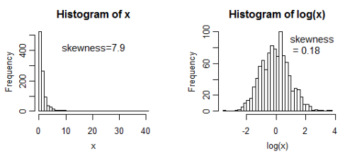
This is one of the most commonly used transformations to address skewed (asymmetrical) data to reduce variability and make your data less skewed. This approach makes it easier to interpret the data and it helps meet the assumption of normality in inferential statistics.

Min-Max Scaling:

The objective of Min-Max scaling is to shift the values closer to the mean of the column. This method scales the data to a fixed range, usually [0, 1] or [-1, 1]. A drawback of bounding this data to a small fixed range is that we will, in turn, end up with smaller standard deviations, which suppresses the weight of outliers in our data.

Standardization (Z-Score Normalization):

Standardization is used to compare features that have different units or scales. This is done by subtracting a measure of location (x- x̅) and dividing by a measure of scale ( σ).

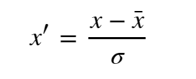
This transforms your data so the resulting distribution has a mean of 0 and a standard deviation of 1. This is method is useful (in comparison to normalization) when we have important outliers in our data and we don’t want to remove them and lose their impact.

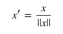
Unit Vector Transformation:

This method uses the Pythagorean Theorem (vx² + vy²=v²) in order to determine the magnitude (hypotenuse) of a vector.

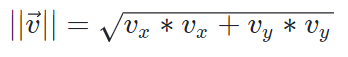
Formula to determine magnitude of vector v

To normalize the vector, we divide each component by the magnitude of the vector in order to scale down to 1. For example, a vector with value 10 divided by 10 equals 1. To scale down to vector size 1, all other components need to be divided by the same amount, 10, as well. So using this method, we can change the length of the vector without affecting the direction.

When performing unit vector transformations, you can create a new variable x’ with a range [0,1].

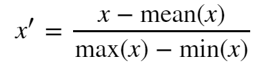
Mean Normalization:

This normalization will create the distribution of features between [-1, 1] by dividing by the standard deviation.

Box Cox Transformation:

Box Cox is used to stabilize the variance (eliminate heteroskedasticity) and transform non-normal dependent variables to a normal shape.

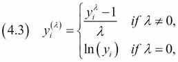
Any value of λ when our datapoint (y) is equal to 1 evaluates to 1. Therefore, when we subtract our datapoint (y^ λ) from 1, we center our transformed data around 0. By dividing by λ, we are normalizing the exponential increase of λ from the numerator.

The boxcox function in Scipy tests a range of λ values and returns the value that makes your data look the most normal. It is also important to note that boxcox only works if all the data is positive and greater than 0, which can be easily achieved by adding a constant (c) to all data before transforming.

These are just a few of the ways we can transform our data. These methods become especially useful and necessary when using machine learning algorithms.

References: