Transfer Learning for Image Classification — (6) Build and Fine-tune the Transfer Learning Model

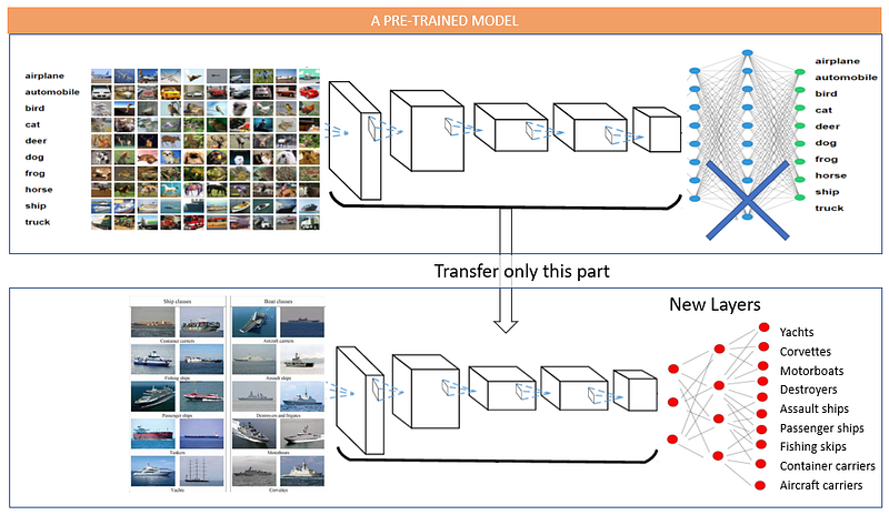
We are ready to apply the transfer learning technique. This chapter will show you how to get the core part from VGG-16 and build a new neural network. You will learn the procedure to build a transfer learning model. It is the same as building any neural network. I will train the model on the car damage images. I will show you how to measure the performance. Finally, I will also show you how to fine-tune a model by opening up more layers. The Python notebook is available via this link.

(A) The VGG-16 Cannot Recognize the Car Damage Images

How good is VGG-16 in recognizing the images of car damages? Our images are of three classes of damages: “car front bumper damage”, “car rear bumper damage”, and “car side damage”. I will feed the model with car damage images. I hope the model can recognize them.

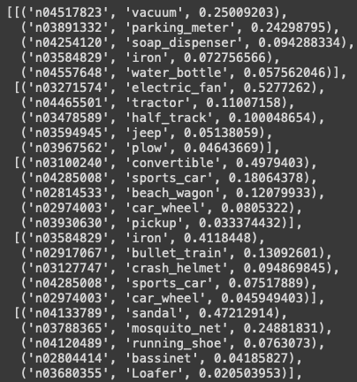
The outputs are kind of amusing. The model predicts the first car image to be a vacuum with 25% and a parking meter with 24%. The model predicts the second image to be an electric fan with 52% and a tractor with 11%. This outcome is expected. It is because the output layer of the pre-trained model does not have the three classes of car damages.

(B) Let’s Build a Transfer Learning Model for the Car Damage Images

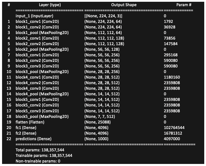
Let me print the content of VGG-16 in Figure (B.1). Layers 1 to 18 are the core layers and Layers 19–22 are the fully connected layers. To apply the transfer learning techniques, we only want the core layers.

(B.0) Remove the Fully Connected Layers of VGG-16

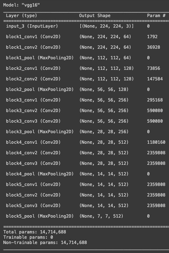
I remove the last three fully connected layers by using include_top=False. Figure (B.2) shows it ends with “block5_pool”.

The procedure to build the transfer learning model is the same as building any neural network. It involves three steps in Keras: (1) .sequential() to build the model architecture, (2) .compile() to compile the model with the loss function and optimization method, and (3) .fit() to train the model. I explain them in (B.1) to (B.3).

(B.1) Build the Model Architecture: .Sequential()

Do you notice the “flatten” layer is dropped? It was in Figure (B.1) but not in Figure (B.2). This layer is important. It converts multi-dimensional arrays into a one-dimensional array, which in turn is fed to the fully connected layers. We need to add a layer that does the same job as the “flatten” layer.

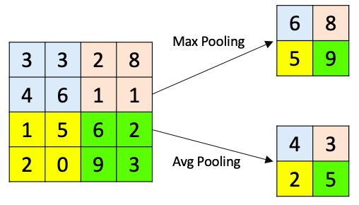
The last layer “block5_pool” outputs 512 feature maps of 7 x 7 pixels. To make the multi-dimensional arrays one-dimensional, I use GlobalAveragePooling2D(). This function computes the average of (height x width) and stacks as a long one-dimensional array as shown in Figure (B.3).

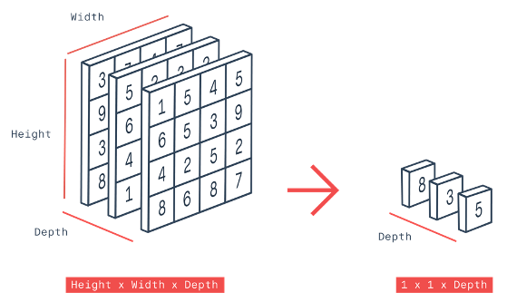
I could have used the “flatten” layer like VGG-16. But here I want to use the “GlobalAveragePooling” layer so I can introduce a new method. The “flatten” and the “GlobalAveragePooling” methods change multi-dimensional arrays to one-dimensional ones. What is the difference? The “flatten” method merely reshapes and stacks the multi-dimensional arrays without changing the values. In contrast, the “GlobalAveragePooling” method derives the averages of the multi-dimensional arrays to get a one-dimensional array. The “flatten” layer will always result in a longer one-dimensional array than that of the GlobalAveragePooling layer. I use GlobalAveragePooling to keep the number of parameters small because there are only three classes in the output layer.

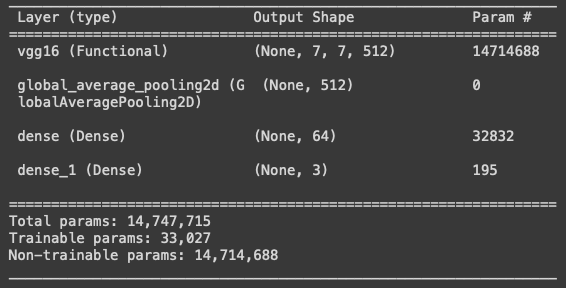
The function.Sequential() defines a neural network structure. It is the pipeline to add any layers to a model. My simple transfer learning model has the following layers:

• VGG16_features
• Global_average_layer
• A regular layer
• Prediction Layer.

The regular layer has 64 neurons. You may want to try a different number of neurons. You may even add more layers or remove this layer. You make this decision based on the performance metrics including loss and accuracy metrics. A simpler model structure is preferred if it can deliver the same performance.

The prediction layer is the output layer that has three neurons. The neurons refer to the three classes. They are the “car front bumper damage”, “car rear bumper damage”, and “car side damage”. The activation='softmax' makes the final predictions between 0 and 1. It is a sigmoid function.

I freeze the layers by trainable=False. It turns all the layer’s weights from trainable to non-trainable. That means the parameters of the frozen layers will not change during model training. The number of trainable parameters is 33,027.

(B.2) Compile the Model: .compile()

The second step of building a neural network is the compiling step. This step defines the evaluation metric and the optimizer. Let me describe them separately.

(B.2.1) The Evaluation Metrics (or called the Loss Function)

An evaluation metric is the loss function that is used to judge the performance of a model. Keras includes almost all the evaluation metrics.

In case you wonder what the appropriate evaluation metric to choose for your model is, let me provide some information. The evaluation metrics belong to three categories: (a) the regression-related metrics, (b) the probabilistic metrics, and (c) the accuracy metrics. The regression-related metrics include mean squared error (MSE), root mean squared error (RMSE), mean absolute error (MAE0, mean absolute percentage error (MAPE), and so on. When your target variable is continuous and you would like to pursue the minimum deviation in terms of percentage errors or absolute errors, you should consider the regression-related metrics.

The probabilistic metrics are considered when your prediction is a probability. They include binary cross-entropy and categorical cross-entropy. If your target is binary, you can use binary cross-entropy. If your target is multi-class, categorical cross-entropy.

The accuracy metrics calculate how often predictions equal labels. The frequently-used metrics are the accuracy class, binary accuracy class, and categorical accuracy class. As the name suggests, the binary accuracy class calculates how often predictions match binary labels, and the categorical accuracy class calculates how often predictions match multiple labels.

Because the image classification problem has multiple classes, I use categorical_crossentropy as the evaluation metric.

(B.2.2) The Optimizers

The optimizer is a function that optimizes a model. Optimizers use the above loss function to calculate the loss of the model and then try to minimize the loss. Without an optimizer, a machine learning model can’t do anything.

The popular optimizers include the Stochastic Gradient Decent (SGD), Resilient Back Propagation (RProp), the Adaptive Moment (Adam), and the Ada family. The SGD is probably the most widely used optimizer. I have included a gentle description in the Appendix. The RProp is widely used in multi-layered feed-forward networks. The Adam is considered more efficient and requires less memory when working with a large amount of data and parameters. It requires less memory and is efficient. I use Adam() as the optimizer. It is a popular stochastic gradient descent method. Its hyper-parameter is the learning rate with a default value of 0.001.

(B.3) Train the Model: .fit()

The third step is the training step. This is a time-consuming step. You will see “epoch 1”, and “epoch 2” appearing on your screen.

In this step, we deal with a unique concept in a neural network called “epoch”. In an epoch, the model goes through all data exactly once. The model parameters are updated in each epoch until they reach optimal values.

If you specify too many epochs, the model will commit overfitting. It will learn the training data too well but predict poorly for a new dataset. How do we determine the optimal number of epochs? The answers are the loss and accuracy metrics. When a model is trained with more epochs, the loss will decrease and the accuracy will increase. After a certain number of epochs, the loss will stop decreasing but increase, and the accuracy decreases. It indicates the model training should end with that epoch. The function EarlyStopping() can be used to monitor and find the optimal number of epochs.

Let me explain the code:

• steps_per_epoch: This is the number of batches. Suppose there are 100,000 images bundled into 32 images per batch, there will be 100,000 / 32 = 3,125 batches. An epoch will go through all 3,125 batches.
• validation_steps: It is the number of batches of the validation data. The validation data should be used all at once. This informs the model that all the batches should be used together for validation. If every epoch only uses some parts of the validation data for validation, you will get different metrics.
• NUM_EPOCHS: This is the number of epochs. Large models require more epochs. Just for our reference. The ResNet model was trained in 35 epochs and the large YOLO model was trained in 160 epochs.
• model.save(): The training can take a long time. It is a good idea to save the completed model.

(C) Model Performance Metrics

Now our model has completed its training. Let me show you how to do the loss and accuracy metrics.

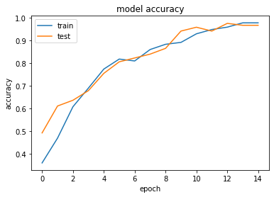
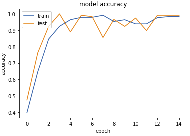
I plot the accuracy metrics for the train and test data.

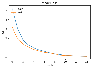
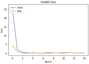
Similarly, I plot the loss metrics for the train and test data.

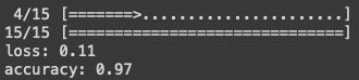
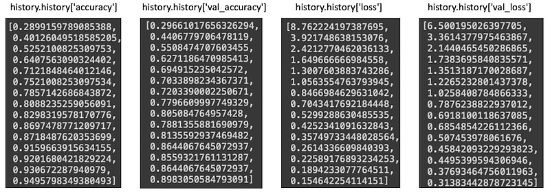
You can print out the accuracy metrics by doing history.history['accuracy'] and history.historyprobabilities['val_accuracy'] for the training and validation data. Likewise, you can get the loss metrics with history.history['loss'] and history.history['val_loss'] . For your reference, below are my outputs.

(D) Model Predictions

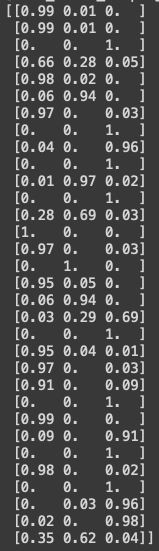
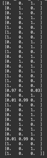
Let’s examine if our model can recognize the 32 images in the first batch of the test data.

For each image, the model predicts the probabilities for the car classes: [‘car_front_bumper_damage’, ‘car_rear_bumper_damage’, ‘car_side_damage’].

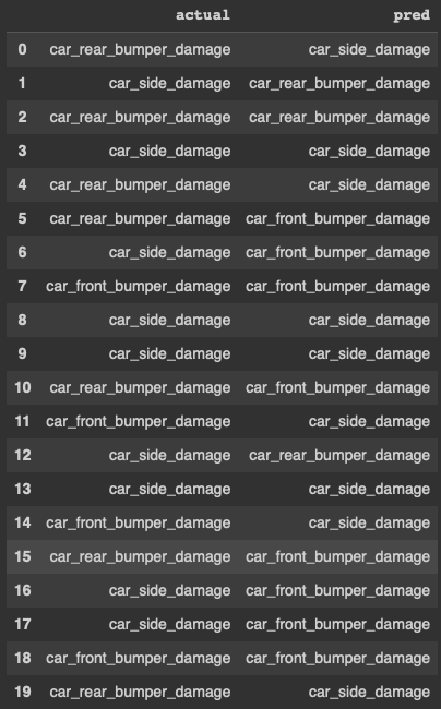
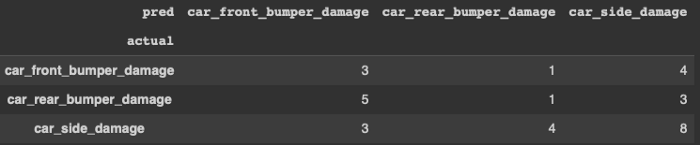
Let me put the actual and predicted values together in a data frame for comparison:

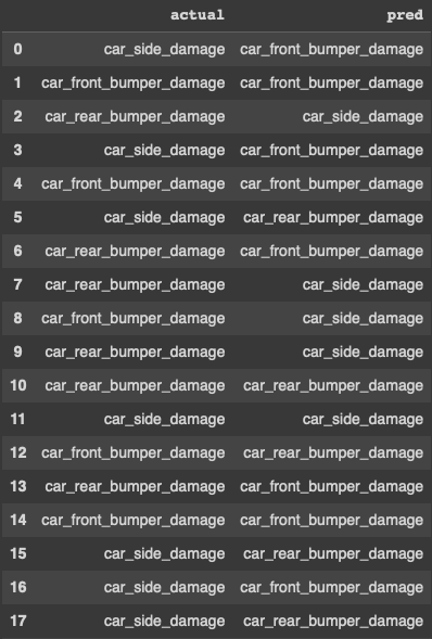
The predictions of the simple transfer learning model are not great, but they are better than the Predictions of VGG-16 for the car damage Images in Figure (A). Below is the confusion matrix for the actual vs. predicted values.

(E) Fine-tune the Model

How can we improve the model performance? To get a better model performance, we can either add more data or work on the model itself (or both). More and better-annotated images should be a good way to improve the model. On the other hand, we can fine-tune the model. Pre-trained models can let users open up more layers for training. A more flexible model can improve the model’s predictability.

(E.1) Open Up More Trainable Layers

Let me name the core VGG-16 “VGG16_trainable” because we will build a new model. To freeze or open a layer is quite easy. We just need to do layer.trainable=False to freeze a layer and layer.trainable=True to open up a layer.

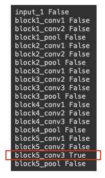
Which layer should we freeze or turn on? A conventional way is to freeze all layers, and then open from the end layers of the model. I freeze all the layers in the following code and then open up the “block5_conv3” layer. This makes 2,359,808 parameters trainable. If we even open the “block5_conv2” layer as well, we will have 2,359,808 + 2,359,808 = 4,719,616 parameters for training. You can open more layers as well.

Do you notice that we do not turn the last layer “black5_pool” to “True”? This is because all the pooling layers have no parameters. As I explained in “Chapter 3: Let’s understand a convolutional neural network”, a pooling layer reduces the resolution of a feature map. It simply downsizes an image and does not have any parameters to be optimized.

(E.2) Build the Fine-tune Model

Our new model has more trainable layers in the core VGG-16. I call the new model “ft_model” because we will fine-tune the model.

(E.3) The Performance Metrics of the Fine-tuned Model

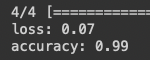
The number of epochs is the same as before. The loss value of the trained model is 0.07, which is better than the loss value of 0.11 in the previous model. I also plot the accuracy and loss metrics.

(E.4) Model Predictions of the Fine-tuned Model

I want to see if this fine-tuned model can recognize the 32 images in the first batch of the test data.

Let me put the actual and predicted values together in a data frame for comparison:

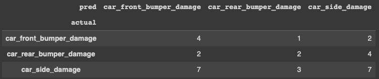
I create a confusion matrix to get more insight into the model performance. This model captures “car side damage” better than other classes. This is the result of opening only one layer “block5_conv3”. Readers are advised to open more layers to test its performance.

Conclusions

In this chapter, we applied the transfer learning techniques to VGG-16 to build the first toy model. We learned how to build, compile and train a neural network model. We also learned how to fine-tune a model by opening up more layers.

This chapter completes the series on transfer learning for image classification. The completion of this book brings me much satisfaction. I hope this series can help your understanding of this topic.

Chapter 1: What is transfer learning?

Chapter 2: The stories of pre-trained models

Chapter 3: Let’s understand a convolutional neural network

Chapter 4: Let’s visualize the pre-trained VGG-16 model layer-by-layer

Chapter 5: Get image data, ready, and go

Chapter 6: Build and fine-tune your transfer learning model

Appendix: How Does the Gradient Descent Work?

The Stochastic Gradient Descent, Gradient Descent, or called SGD, is probably the most popular optimization algorithm. It is a first-order iterative optimization algorithm for finding the minimum.

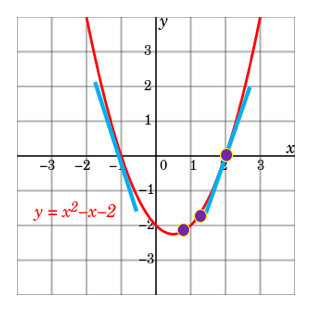
Let me show you how it works with a parabola function y=x²-x-2. To find the x value that minimizes y=x²-x-2, all you need to do is to set the first-order derivative to zero: dy/dx=2x-1=0. This is the same as saying the slope is zero at x=1/2. It is super easy, isn’t it?

But what if you do not or cannot find the exact point where the slope is zero? You can use a numeric approach called “gradient descent”. It starts with any randomly picked number on the parabola. Let’s do some math step by step to see how it approaches the optimal value.

• Suppose it is x=3. At that point, the slope and y values are dy/dx=2x-1=2∗3–1=5 and y=4 respectively. The value of the slope is positive, meaning as x increases y will increase.
• Let’s take another random x on the parabola. Suppose it is x = -3, the slope and y value are dy/dx=2x-1=2∗(-3)-1=-7 and y=10 respectively. The derivative tells us we are getting closer or away from the minimum.
• Since we want to minimize y, it should go in the opposite direction. That’s why it is called “descent”. You can have a gradient ascent if it is in the same direction.
• We set the iteration in Equation (1) such that the next x is the current x minus the slope. The ⍵ is the step length or called the learning rate (lr). It can take any value. A small ⍵ value means every step is a small step, which takes a longer time to approach zero.

Readers are recommended to purchase books by Chris Kuo:

• The explainable AI: https://a.co/d/cNL8Hu4
• Transfer learning for image classification: https://a.co/d/hLdCkMH
• Modern time series anomaly detection: https://a.co/d/ieIbAxM
• Handbook of Anomaly Detection: https://a.co/d/5sKS8bI