Summary

This article introduces a multi-part tutorial on building an interpretable Temporal Fusion Transformer (TFT) model for high-frequency stock price prediction, including confidence intervals for risk management.

Abstract

The tutorial, aimed at educating readers on the creation of a predictive model for 1-minute stock prices, emphasizes the importance of understanding the inherent uncertainty in stock price prediction. It provides a comprehensive guide from data collection and preprocessing to exploratory data analysis (EDA) and feature engineering. The author collects a substantial dataset of over 1,500 stocks with 1-minute intraday data for a six-month period and demonstrates the process of data cleaning, resampling, and filtering for liquidity. The article underscores the use of confidence intervals to assess prediction risk and outlines the initial steps taken to prepare data for a machine learning model, setting the stage for subsequent parts of the series that will delve into model training and evaluation.

Opinions

The author acknowledges the speculative nature of stock price prediction and cautions against relying on the model for actual trading decisions.
There is an emphasis on the model's ability to identify high probability moves rather than striving for perfect prediction accuracy, aligning with the realistic approach to trading where reward-to-risk ratios are critical.
The tutorial is not intended to provide financial advice but rather to serve as an educational resource for those interested in applying machine learning to finance.
The author suggests that even with a predictive accuracy of 50%, a trading strategy can be profitable if it effectively manages risk and focuses on high reward-to-risk trades.
By focusing on precision and using confidence intervals, the TFT model is presented as a valuable tool for informed trading decisions, despite the unpredictable nature of financial markets.

Training a Transformer Model to Predict 1-Minute Stock Prices: Tutorial with Code Samples (Part 1)

Discover How to Build an Interpretable Transformer Model for High-Frequency Stock Price Prediction, with Confidence Intervals for Risk Management.

Disclaimer: Stock price prediction is inherently uncertain, and this tutorial is intended for educational purposes only. The model and methods discussed here should not be interpreted as financial advice or relied upon for actual trading decisions. While the Temporal Fusion Transformer (TFT) model provides confidence intervals that can help assess risk, no model can fully account for the unpredictable nature of financial markets. Always conduct thorough research and consult with financial professionals before making investment decisions.

Welcome to this multi-part series on building an interpretable model for high-frequency stock price prediction using the Temporal Fusion Transformer (TFT). Throughout this series, we’ll dive deep into the steps of training a model capable not only of predicting stock prices but also of providing confidence intervals that make it a valuable tool for risk assessment. From data collection and preprocessing to model training, evaluation, and interpretation, each post will guide you through a critical stage of the process.

In this first part, we’ll start with the fundamentals: gathering the right data and performing exploratory data analysis (EDA) to understand the trends, patterns, and potential pitfalls in high-frequency stock data.

This tutorial assumes you already have historical 1-minute bar data available in your environment. If you don’t have this data yet, be sure to check out my post on how to download it for free here (note: if you want me to send you the raw data file, contact me privately).

Background and Motivation

The stock market is a dynamic and often unpredictable environment. Successful intraday traders rely not just on predictions but on high reward-to-risk trades. Even if a trader only correctly predicts the direction of a stock 50% of the time, they can still be profitable if the average reward per trade outweighs the average risk. Automated trading algorithms help traders remove emotions from trading, making it possible to focus on technical indicators and systematic decision-making.

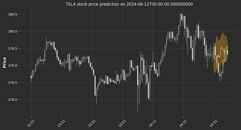
With our Temporal Fusion Transformer model, the goal isn’t to achieve perfect prediction accuracy (an impossible feat in financial markets) but to develop a model that can identify high probability moves while assessing the risk associated with each prediction. By focusing on precision and using confidence intervals, the model can serve as a valuable tool for making more informed trading decisions.

Data Collection and Preparation

For this project, I collected 1-minute intraday data for stocks with an average daily trading volume exceeding 1 million. This dataset covers a 6-month period from January 1, 2024, to July 11, 2024, totaling over 1,500 stocks. For each stock, I gathered the standard OHLCV (Open, High, Low, Close, Volume) data, capturing each price movement throughout the trading day. To simplify the data handling process, I saved this data in a single .parquet file for efficient access and analysis.

Data Loading and Initial Cleaning

In the Jupyter Notebook, I start by importing essential libraries for data manipulation, visualization, and modeling. Here’s an example of some of the libraries used:

import pandas as pd
import yfinance as yf
import matplotlib.pyplot as plt
import numpy as np
import seaborn as sns
from datetime import datetime

then load the dataset and set the date as the index for time-based analysis:

df = pd.read_parquet("data.parquet")
df.set_index("datetime", inplace=True)
df.sample(10) # print 10 random rows from the dataset

output:

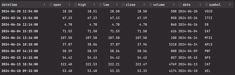
To see how much data I am dealing with, I use df.info() to get this information:

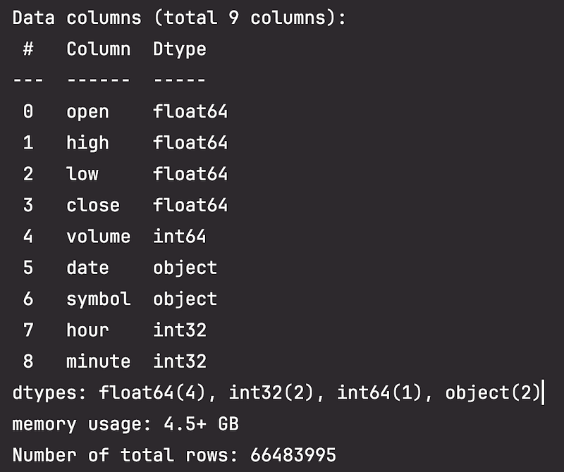
So this dataframe is quite big, containing over 66 million rows and using over 4.5 GB of memory. To make it more manageable and filter out stocks that are not very liquid, I use “Stock Average Nominal Volume” which is calculated as the median daily volume multiplied by the average price. I keep only the top 100 stocks by average nominal volume.

def resample_to_daily(group):
    resampled_group = group.resample('D').agg({
        'open': 'first',
        'high': 'max',
        'low': 'min',
        'close': 'last',
        'volume': 'sum'
    }).dropna()
    return resampled_group

# Apply the resampling function to each group
df_daily = df.groupby('symbol').apply(resample_to_daily).reset_index()
df_daily["stock_median_volume"] = df_daily.groupby("symbol")["volume"].transform("median").astype(int)
df_daily["stock_average_price"] = df_daily.groupby("symbol")["close"].transform("mean")
df_daily["stock_average_nominal_volume"] = df_daily["stock_median_volume"] * df_daily["stock_average_price"]
top_100_symbols = df_daily.groupby("symbol")['stock_average_nominal_volume'].median().nlargest(100).index
# Filter the DataFrame to keep only the top 100 stocks by nominal volume
df_daily = df_daily[df_daily['symbol'].isin(list(top_100_symbols))]
df = df[df['symbol'].isin(list(top_100_symbols))]
print(f"Number of total one minute bars after resampling: {df.shape[0]}")
print(f"Symbols: {df_daily.symbol.unique()}")

Number of total one minute bars after resampling: 5165367
Symbols: ['AAL' 'AAPL' 'ABBV' 'ABNB' 'ABT' 'ADBE' 'AMAT' 'AMD' 'AMZN' 'ANET' 'AVGO'
 'AXP' 'BA' 'BAC' 'BMY' 'C' 'CAT' 'CCL' 'CLSK' 'CMCSA' 'COIN' 'COP' 'COST'
 'CRM' 'CRWD' 'CSCO' 'CVNA' 'CVS' 'CVX' 'DAL' 'DELL' 'DHR' 'DIS' 'DKNG'
 'ENPH' 'F' 'FCX' 'GE' 'GEV' 'GM' 'GOOG' 'GOOGL' 'GS' 'HD' 'IBM' 'INTC'
 'JNJ' 'JPM' 'KO' 'LLY' 'MA' 'MARA' 'MCD' 'MDLZ' 'MDT' 'META' 'MRK' 'MRVL'
 'MS' 'MSFT' 'MSTR' 'MU' 'NEE' 'NEM' 'NFLX' 'NKE' 'NOW' 'NVDA' 'ORCL'
 'OXY' 'PANW' 'PEP' 'PFE' 'PG' 'PLTR' 'PM' 'PYPL' 'QCOM' 'RIVN' 'RTX'
 'SBUX' 'SCHW' 'SMCI' 'SNOW' 'SOFI' 'SQ' 'T' 'TGT' 'TJX' 'TMO' 'TMUS'
 'TSLA' 'TXN' 'UBER' 'UNH' 'V' 'VRT' 'WFC' 'WMT' 'XOM']

EDA and Feature Engineering

In the next step, I conduct exploratory data analysis (EDA) to understand the key characteristics of our filtered dataset and begin feature engineering to extract relevant indicators. By visualizing trends, price distributions, and volume changes, I aim to uncover patterns and insights that may guide our predictive model.

This brings us to the end of Part 1. In the following part, we’ll dive deeper into feature engineering and begin preparing our dataset for model training.

If you’re excited about building machine learning models for stock prediction, make sure to follow me for the latest updates in this series! Each post will walk you through a new stage, from data preparation to model evaluation and strategy backtesting, with hands-on code and insights tailored for finance enthusiasts and aspiring quants — hit that follow button and stay tuned!