Train-Test Split in Python: A Step-by-Step Guide with Example for Accurate Model Evaluation

If you’re new to machine learning, you’ve likely encountered the train-test split method. This fundamental technique divides a dataset into two parts to evaluate a model’s performance on unseen data.

Understanding Train-Test Split

Train-Test Split is a technique in machine learning where a dataset is divided into two subsets and allows you to simulate how your model would perform with new data.

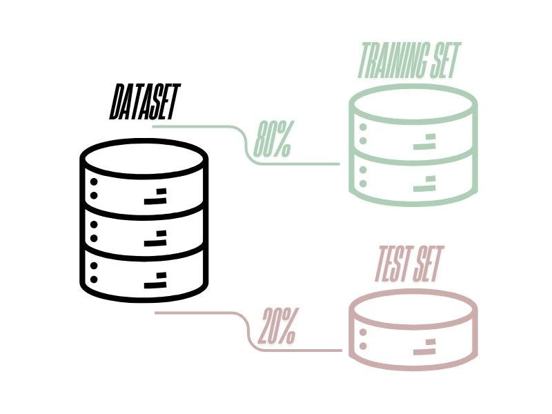
The train-test split method divides your dataset into two main parts:

Training Set: Used to train the model and help it learn patterns.

Test Set: Used to evaluate how well the model generalizes to new data.

But how to choose the right amount for each set from the dataset?

A common approach is to split the dataset into 80% training set and 20% testing set, though 70–30 or 60–40 splits are also used based on the dataset size.

In this article we are going to use an example to explain with few steps in Python code how this method works and generate two models for predictions using Scikit-learn library in Python and evaluate them to have a better opinion about how good our predictions are.

Step-by-Step Implementation in Python

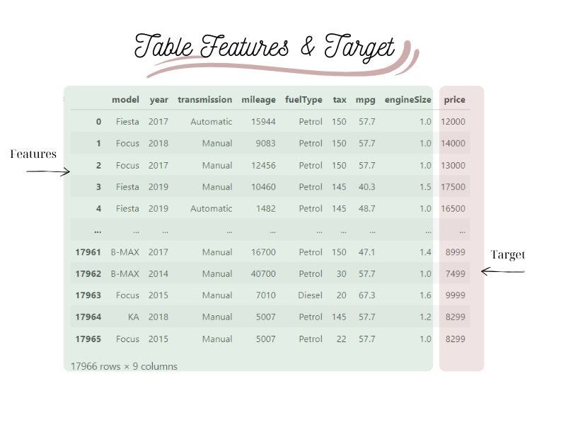
Our dataset contains informations about the model, year, transmision, mileage, fuel type, tax, mpg, engine size and the price of each car.

Our Goal: Using this dataset to build a model that can learn patterns from data and make predictions about the price of the car.

That means that our target is price and all the other columns of our dataset will be the features.

Dataset Preparation

Our first priority is to clean our dataset to improve data quality and provide more accurate, consistent and reliable information for decision-making. It is important not to overlook this step from our process. Otherwise we will have overfitting or underfitting, resulting in a model that can’t make accurate predictions or conclusions from any data other than the training data.

If you are not familiar with the above steps make sure to spend time and learn about those ideas first and then you can get back to creating a model.

As this is not the subject of this article I am skiping the cleaning process but you can find all my code here. If you have questions about it feel free to ask me!

Preparing Dataset for Machine Learning

1. Import Required Libraries.

# import required libraries
import pandas as pd 
import matplotlib.pyplot as plt
import sklearn
from sklearn.ensemble import RandomForestRegressor
from sklearn.preprocessing import StandardScaler, LabelEncoder
from sklearn import linear_model
from sklearn.model_selection import train_test_split

2. Separate the target value from the features

Delete the “price” column from the dataset and create a y parameter with this column.

# separate features from target value
X=df.drop(['price'],axis=1)
y=df['price']
X

3. Encode Categorical Data

In order to make a machine learning prediction, you have to encode all your categorical columns to numerical. In this example we have 3 object columns (“model”, “transmission”, “fuelType”). Below you can observe which numbers replaced each unique categorical value.

# encode categorical data
le=LabelEncoder()
list=['model','transmission','fuelType']
for i in list:
  X[i]=le.fit_transform(X[i])
  print("Unique categorical values for",i,":", df[i].unique())
  print("Unique numerical values for",i,":", X[i].unique())
  print("")

Output:
Unique categorical values for model : [' Fiesta' ' Focus' ' Puma' ' Kuga' ' EcoSport' ' C-MAX' ' Mondeo' ' Ka+'
 ' Tourneo Custom' ' S-MAX' ' B-MAX' ' Edge' ' Tourneo Connect'
 ' Grand C-MAX' ' KA' ' Galaxy' ' Mustang' ' Grand Tourneo Connect'
 ' Fusion' ' Ranger' ' Streetka' ' Escort' ' Transit Tourneo' 'Focus']
Unique numerical values for model : [ 5  6 16 13  2  1 14 12 21 18  0  3 20  9 11  8 15 10  7 17 19  4 22 23]

Unique categorical values for transmission : ['Automatic' 'Manual' 'Semi-Auto']
Unique numerical values for transmission : [0 1 2]

Unique categorical values for fuelType : ['Petrol' 'Diesel' 'Hybrid' 'Electric' 'Other']
Unique numerical values for fuelType : [4 0 2 1 3]

4. Split your Dataset

Now it’s time to proceed to train-test split method.

Choose a Split Ratio: Decide how much data to allocate to training and testing. For example, an 80–20 split. Random Selection: Randomly shuffle the data before splitting to avoid any order or pattern that could bias the model. Allocate Data: Assign the selected ratio for training and the remainder for testing.

#Performing train_test_split
X_train,X_test,y_train,y_test=train_test_split(X,y,test_size=0.2, shuffle=True, random_state=42)
print(X_train.shape, y_train.shape)
print (X_test.shape, y_test.shape)

IMPORTANT NOTE! random_state is a parameter in train_test_split that controls the random number generator used to shuffle the data before splitting it. In other words, it ensures that the same randomization is used each time you run the code, resulting in the same splits of the data. So, make sure you are using it as it is an important part of your split data. Otherwise, each time will be generated another dataset and it might not reproduce the results of your experiments, your findings may not be reliable. By setting “random_state,” you ensure that the results of your experiments are reproducible, even if you rerun the code several times. Also we are going to compare below the performance of two machine learning models using different algorithms or hyperparameters. By setting “random_state,” we ensure that the models are trained and tested on the same data, making it easier to compare their performance.

Building and Evaluating Models

1. Linear Regression Model

# Instantiate the linear regression model
lin_model = linear_model.LinearRegression()
# Fit the linear regression model
lin_model.fit(X_train, y_train)
# Prediction on Test Data
y_pred_l = lin_model.predict(X_test)

#predict the price of a car:
predictedprice = lin_model.predict([[5, 2017, 0, 15000, 3, 150, 57, 1.5]])

print(predictedprice.round(2))

Output:

[13819.6]

After creating our model we used some random data to check the output. But how good is this predicted price?

It is a crucial step to evaluate your model to check how good its predictions are.

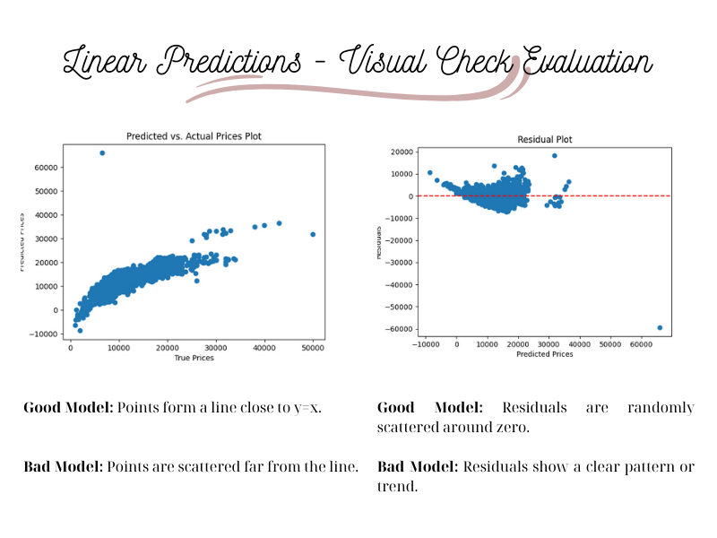
You can do that by creating a scatter plot using the predicted prices (y_pred_l) that you created above and the actual prices (y_test) of the test data.

Evaluation

# Predicted vs. Actual Plot
plt.scatter(y_test, y_pred_l)
plt.xlabel("True Prices")
plt.ylabel("Predicted Prices")
plt.title('Predicted vs. Actual Prices Plot')
plt.savefig('Predicted vs. Actual Prices Plot-Linear.png')

# Predicted vs. Actual Plot
# Residual Plot
residuals = y_test - y_pred_l
plt.scatter(y_pred_l, residuals)
plt.xlabel('Predicted Prices')
plt.ylabel('Residuals')
plt.title('Residual Plot')
plt.axhline(y=0, color='r', linestyle='--')
plt.savefig('Residual Plot-linear.png')
plt.show()

As we can observe our predictions are not bad but there is room for improvement. There are different performance metrics that can be used to measure the goodness of your model. Here as an example we will use R-squared. The closer the R-squared is to 1 the better is your model predictions.

# Measure Score
print("Score for Linear Regression Model is:", lin_model.score(X_test, y_test).round(2))

Output:

Score for Linear Regression Model is: 0.71

0,71 is not bad but is not very good either, so let’s find another method (Forest Regression) to predict our prices.

2. Forest Regression Model

# Instantiate the RandomForestClassifier
forest_model = RandomForestRegressor(n_estimators=100)
# Fit the RandomForestClassifier
forest_model.fit(X_train,y_train)
# prediction on Test Data
y_pred_f = forest_model.predict(X_test)

Evaluation

# Predicted vs. Actual Plot
plt.scatter(y_test, y_pred_f)
plt.xlabel("True Prices")
plt.ylabel("Predicted Prices")
plt.title('Predicted vs. Actual Prices Plot')
plt.savefig('Predicted vs. Actual Prices Plot-Forest.png')

# Residual Plot
residuals = y_test - y_pred_f
plt.scatter(y_pred_f, residuals)
plt.xlabel('Predicted Prices')
plt.ylabel('Residuals')
plt.title('Residual Plot')
plt.axhline(y=0, color='r', linestyle='--')
plt.savefig('Residual Plot-Forest.png')
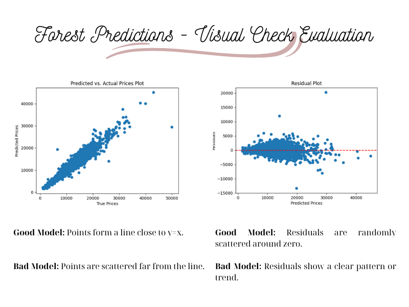
plt.show()

The scatter plots now are much better. Let’s check the R-squared.

# Measure Score
print("Score for Forest Regression Model is:", forest_model.score(X_test, y_test).round(2))

Output:

Score for Forest Regression Model is: 0.93

Comparison and Conclusion

• Linear Regression (R² = 0.71): Works but is less accurate due to limitations in capturing complex patterns.
• Random Forest Regression (R² = 0.93): Performs significantly better due to its ability to handle non-linearity and interactions between variables.

By mastering the train-test split method and model evaluation techniques, you can improve the accuracy of your machine learning models and make informed decisions about algorithm selection.

Experimenting with different splits and models will further enhance predictive performance.

Thanks for reading! If you found this article helpful at all give it a clap!