
Total Least Squares in comparison with OLS and ODR
The holistic overview of linear regression analysis

Table of contents:
- OLS: quick review
- TLS: explanation
- ODR: scratching the surface
- Comparison of three methods and analyzing the results
Total least squares(aka TLS) is one of regression analysis methods to minimize the sum of squared errors between a response variable(or, an observation) and a predicated value(we often say a fitted value). The most popular and standard method of this is Ordinary least squares(aka OLS), and TLS is one of other methods that take different approaches. To get a practical understanding, we’ll walk through these two methods and plus, Orthogonal distance regression(aka ODR), which is the regression model that aims to minimize an orthogonal distance.
OLS: quick review
To brush up our knowledge, first let’s review regression analysis and OLS. In general, we use regression analysis to predict(or simulate) future events. To be more precise, if we have a bunch of data collected in the past(which is an independent variable) and also corresponding outcomes(which is a dependent variable), we can make the machine that predicts future outcomes with our new data that we just collected.
To make a better machine, we apply regression analysis and try to get better parameters, which is a slope and a constant for our models. For instance, let’s take a look at the figure below. We seek parameters of the red regression line(and blue points are data points (response variables and independent variables), and the length of grey line is the amount of the residual calculated by this estimator).
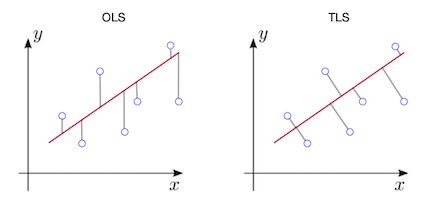
In OSL, the gray line isn’t orthogonal. This is the main and visually distinct difference between OSL and TLS(and ODR). The gray line is parallel to the y-axis in OSL, while it is orthogonal toward the regression line in TLS. The objective function (or loss function) of OLS is defined as:
Which is solved by a quadratic minimization. And we can get parameter vectors from that(this is all what we need).
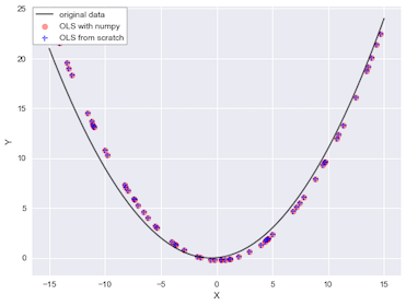
Numpy provides numpy.linalg.lstsq for this though, it’s easy to implement this normal equation from scratch. We get parameter vectors in b in codes below and use it to predict fitted values. numpy.linalg.lstsq expects the constant c exists at a last index, so we need to switch the position of column values.
TLS: explanation
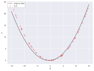
Let’s back to TLS and consider the reason TLS is preferred over OLS. OLS expects that the all sample data is measured exactly, or observed without error. However, in real case there are more or less observational errors. If the assumption is reasonable, OLS could be an inconsistent estimator, and not the ideal machine that theory assumes. TLS can take the problem into consideration, and it allows that there are errors in both independent and dependent variables. We want to minimize errors E, for an independent variable and errors F for a dependent variable. Those errors are considered as to contain both an observational error and a residual.

After solving a covariance matrix of X and Y with SVD, we ended up getting the equation below. U is the left singular vectors of XᵀY and Σ is the diagonal matrix with singular values on its diagonal.
Also the parameter vectors B is defined as:
In the codes below(implementation of TLS normal equation), we calculate the [E F] and add the return to Xtyt. (Xtyt is just meant x tilde and y tilde. A tilde often implies an approximate value) The vertically stacked vectors [Vxy Vyy] is the whole last column of right singular vectors of XᵀY, V. The Vxy and Vyy, which is used for the calculation of parameter vectors B, are different from those. Vxy and Vyy are truncated the number of X variables.
The first n columns are for errors E, and n to last column for errors F. We can also calculate the estimate Y value through Y=[X, E]B, which is written in the line 15 below. For a reference of more mathematical processes and codes in Matlab, we can check this detailed pdf.
(Caveat: for non Matlab, R, Julia, nor Fortran users, an index of array begins from 1)
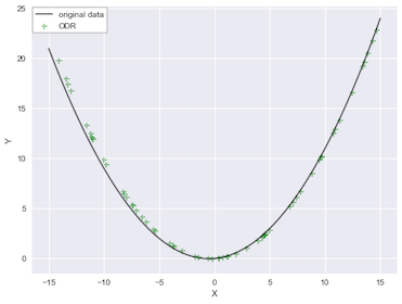
ODR: scratching the surface
There is the regression model that aims to minimize an orthogonal distance. Thankfully, Scipy provides scipy.odr package. We can set the error values wd and we in the Data function. This is for a weight matrix to address an unequal variance of residuals(heteroscedasticity). If we know how big/small the errors are beforehand, this tweak can improve the estimator. In the real world, however, it’s hard to determine or estimate that. This weighting is also the one of effective ways to improve the application of Weighted Least Squares and Generalized Least Squares.
We set 1× N array of error values in wd, which means ith error value is applied to ith data point.
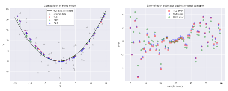
ODR fits better than others for this data set.
Comparison of three methods
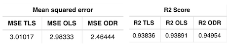
Let’s compare all of three methods and see their fitness visually. The gray upper triangle in the left figure is the data that contains errors in both an independent variable and a dependent variable. The right figure shows errors of each data point produced by each model. The vertical axis indicates how big errors are. ODR and TLS fit very well on the center of the quadratic curve, however, as far away off the center they move, their prediction loss the precision. To interpret that, ODR and TLS work well when the variance of fitted values are small. Especially when the variance of fitted values are so large, TLS won’t work correctly any longer, though it is very precise to predict fitted values without any weighting values when the variance is small. In which case, we would need to apply iteration methods, such as gradient descent.
To make sure mean sum of squared error(aka MSE) and Goodness-of-fit(or R2 score) for each model. Overall, ODR fits better in this data sample though, it depends on the data. We will need to consider these models one by one until we find the best model.
References:
Total Least Squares PDF CEE 629 Duke University
Primer on Orthogonal Distance Regression
The sample data that we walked through:


