Top 3 Methods for Handling Skewed Data

Real-world data can be messy. Even some learning datasets contain attributes that need severe modifications before they can be used to do predictive modeling.

And that’s fine.

Let’s take a linear regression model for example. You probably know this already, but the model makes a good amount of assumptions for the data you provide, such as:

1. Linearity: assumes that the relationship between predictors and target variable is linear
2. No noise: eg. that there are no outliers in the data
3. No collinearity: if you have highly correlated predictors, it’s most likely your model will overfit
4. Normal distribution: more reliable predictions are made if the predictors and the target variable are normally distributed
5. Scale: it’s a distance-based algorithm, so preditors should be scaled — like with standard scaler

That’s quite a lot for a simple model. Today I want to focus on the fourth point, and that is that predictors and target variable should follow a gaussian distribution.

Now that’s not always quite possible to do, ergo you cannot transform any distribution into a perfect normal distribution, but that doesn’t mean you shouldn’t try.

To start out, let’s load a simple dataset and do the magic.

The Dataset

I will use the familiar Boston Housing Prices dataset to explore some techniques of dealing with skewed data.

There’s no need to download it, as you can import it straight from Scikit-learn. Here’s the code with all the imports and dataset loading:

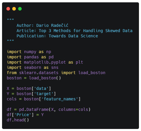
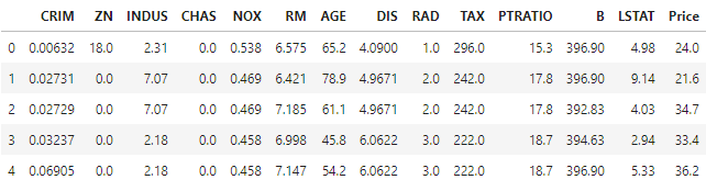
Upon execution the first couple of rows will be shown, you should have the same output as I do:

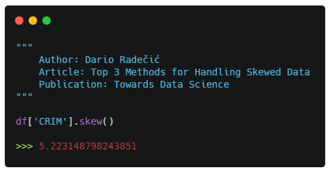
I don’t want to explore all of the variables as I’ve done some tests before and concluded that the variable CRIMhas the highest skew. Here’s the code to verify my claim:

Cool. Now you can use the Seaborn library to make a histogram alongside with the KDE plot to see what we’re dealing with:

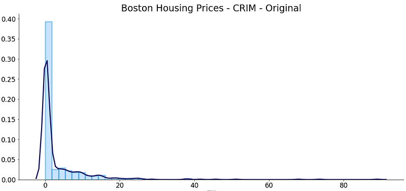
This certainly doesn’t follow a normal distribution. And yeah, if you’re wondering how I shifted from awful-looking default visualization, here’s an article you should read:

Okay, now when we have that covered, let’s explore some methods for handling skewed data.

1. Log Transform

Log transformation is most likely the first thing you should do to remove skewness from the predictor.

It can be easily done via Numpy, just by calling the log() function on the desired column. You can then just as easily check for skew:

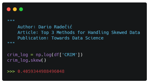
And just like that, we’ve gone from the skew coefficient of 5.2 to 0.4. But before jumping to conclusions we should also make a quick visualization:

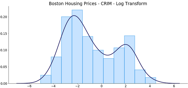
Well, it’s not normally distributed for sure, but is a lot better than what we had before!

As you would expect, the log transformation isn’t the only one you can use. Let’s explore a couple of more options.

2. Square Root Transform

The square root sometimes works great and sometimes isn’t the best suitable option. In this case, I still expect the transformed distribution to look somewhat exponential, but just due to taking a square root the range of the variable will be smaller.

You can apply a square root transformation via Numpy, by calling the sqrt() function. Here’s the code:

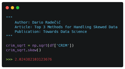
The skew coefficient went from 5.2 to 2, which still is a notable difference. However, the log transformation ended with better results.

Nevertheless, let’s visualize how everything looks now:

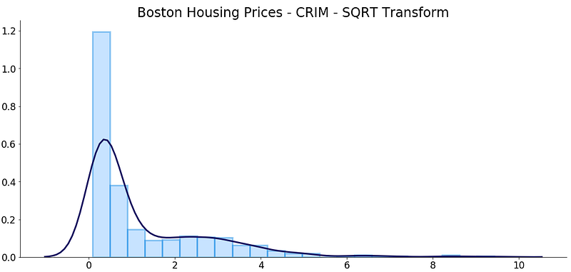
The distribution is pretty much the same, but the range is smaller, as expected.

Before declaring the log transformation as the winner, let’s explore one more.

3. Box-Cox Transform

This is the last transformation method I want to explore today. As I don’t want to drill down into the math behind, here’s a short article for anyone interested in that part.

You should only know that it is just another way of handling skewed data. To use it, your data must be positive — so that can be a bummer sometimes.

You can import it from the Scipy library, but the check for the skew you’ll need to convert the resulting Numpy array to a Pandas Series:

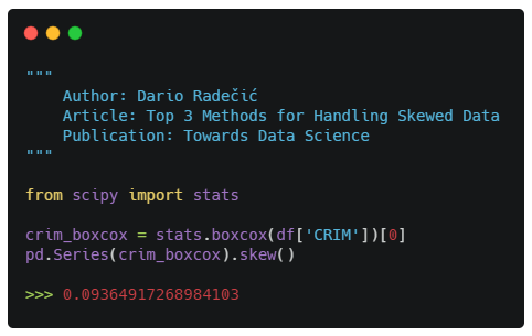
Wow! The skew dropped from 5.2 to 0.09 only. Still, let’s see how the transformed variable looks like:

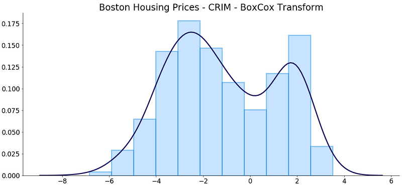
The distribution is pretty similar to the one made by the log transformation, but just a touch less bimodal I would say.

Before you go

Skewed data can mess up the power of your predictive model if you don’t address it correctly.

This should go without saying, but you should remember what transformation you’ve performed on which attribute, because you’ll have to reverse it once when making predictions, so keep that in mind.

Nevertheless, these three methods should suit you well.

What transformation methods are you using? Please let me know.

Loved the article? Become a Medium member to continue learning without limits. I’ll receive a portion of your membership fee if you use the following link, with no extra cost to you.