Top 10 Machine Learning Algorithms for 2024

Essentials of machine learning algorithms with implementation in Python

In simple terms, a machine learning algorithm is a blueprint that allows computers to learn and make predictions from data. Instead of explicitly telling the computer what to do, we provide the algorithm with a large amount of data and allow it to discover patterns, relationships, and insights for itself.

in this guide i will give you a comprehensive understanding of Top 10 machine learning algorithm and provide code examples in Python. If you want to start building your own machine learning projects, this guide is for you.

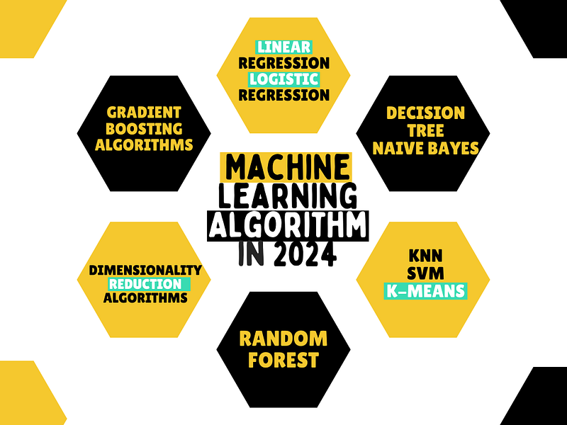
List of Top 10 Common Machine Learning Algorithms

Here is the list of commonly used machine learning algorithms. These algorithms can be used to solve practically any data problem.

1. Linear Regression
2. Logistic Regression
3. Decision Tree
4. SVM
5. Naive Bayes
6. kNN
7. K-Means
8. Random Forest
9. Dimensionality Reduction Algorithms
10. Gradient Boosting algorithms

• GBM
• XGBoost
• LightGBM
• CatBoost

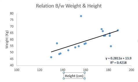
1. Linear Regression

Concept: Linear Regression is used to predict a continuous outcome (like predicting a person’s weight based on their height). It assumes a linear relationship between the input features (independent variables) and the target variable (dependent variable).

Mathematical Explanation:

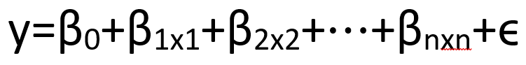
• y is the predicted value.
• x1,x2,…,xn are the input features.
• β0,β1,…,βn are the coefficients (parameters) that the model learns.
• ϵ is the error term (the difference between the actual and predicted value).

There are several ways to determine the goodness of fit of a linear regression model:

The goal is to find the coefficients (β values) that minimize the sum of squared errors (the differences between actual and predicted values).

R-squared: R-squared is a statistical measure that represents the proportion of the variance in the dependent variable that is explained by the independent variables in the model. An R-squared value of 1 indicates that the model explains all the variance in the dependent variable, and a value of 0 indicates that the model explains none of the variances.

Adjusted R-squared: Adjusted R-squared is a modified version of R-squared that accounts for the number of independent variables in the model. It is a better indicator of the model’s goodness of fit when comparing models with different numbers of independent variables.

Root Mean Squared Error (RMSE): RMSE measures the difference between the predicted values and the actual values. A lower RMSE indicates a better fit of the model to the data.

Mean Absolute Error (MAE): MAE measures the average difference between the predicted values and the actual values. A lower MAE indicates a better fit of the model to the data.

Code Example:

from sklearn.datasets import make_regression
from sklearn.linear_model import LinearRegression
from sklearn.model_selection import train_test_split

# Create a synthetic dataset
X, y = make_regression(n_samples=100, n_features=1, noise=0.1, random_state=42)

# Split the data into training and testing sets
X_train, X_test, y_train, y_test = train_test_split(X, y, test_size=0.2, random_state=42)

# Create and train the model
model = LinearRegression()
model.fit(X_train, y_train)

# Make predictions
y_pred = model.predict(X_test)

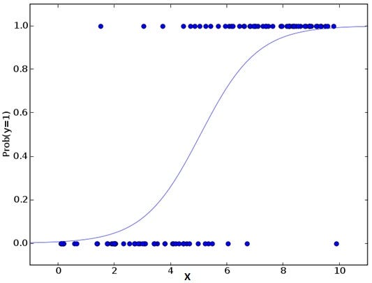
print("Predictions:", y_pred)

2. Logistic Regression

Concept: Logistic Regression is used for binary classification problems, where the outcome is categorical (like predicting whether an email is spam or not). Instead of predicting a continuous value, it predicts the probability that a given input belongs to a certain class.

Mathematical Explanation:

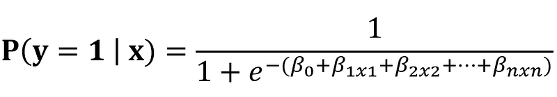
• P(y=1∣x) is the probability that the outcome y is 1 (e.g., spam).
• e is the base of the natural logarithm.
• The rest of the terms are similar to Linear Regression, but they are transformed using the logistic function to keep the output between 0 and 1.

Code Example:

from sklearn.datasets import load_breast_cancer
from sklearn.linear_model import LogisticRegression
from sklearn.model_selection import train_test_split

# Load the breast cancer dataset
X, y = load_breast_cancer(return_X_y=True)

# Split the data into training and testing sets
X_train, X_test, y_train, y_test = train_test_split(X, y, test_size=0.2, random_state=42)

# Create and train the model
model = LogisticRegression(max_iter=10000)
model.fit(X_train, y_train)

# Make predictions
y_pred = model.predict(X_test)

print("Predictions:", y_pred)

3. Decision Tree

Concept: Decision trees are a type of machine learning algorithm used for both classification and regression tasks. They are a powerful tool for decision making and can be used to model complex relationships between variables.

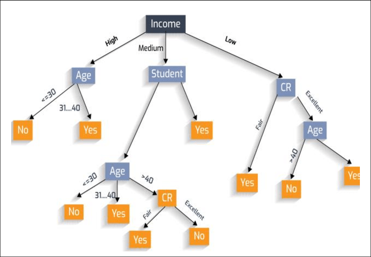
A decision tree is a tree-like structure, with each internal node representing a decision point, and each leaf node representing a final outcome or prediction. The tree is built by recursively splitting the data into subsets based on the values of the input features. The goal is to find splits that maximize the separation between the different classes or target values.

The process of building a decision tree begins with selecting the root node, which is the feature that best separates the data into different classes or target values. The data is then split into subsets based on the values of this feature, and the process is repeated for each subset until a stopping criterion is met. The stopping criterion can be based on the number of samples in the subsets, the purity of the subsets, or the depth of the tree.

Mathematical Explanation:

• The splitting is based on criteria like Gini impurity or Information Gain:

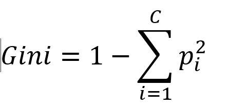
• Gini Impurity: Measures how often a randomly chosen element from the set would be incorrectly classified. pi is the probability of choosing an element of class iii out of C classes.
• Information Gain: Measures the reduction in entropy after the dataset is split on a feature. It’s the difference between the entropy before and after the split.

There are some common challenges with decision trees. One key issue is their tendency to overfit data, especially when the tree gets deep and branches out extensively. Overfitting occurs when the tree becomes too complex, capturing noise instead of actual patterns. This can hurt its performance on new, unseen data. But worry not! We have tricks like pruning, regularization, and cross-validation up our sleeves to keep overfitting in check.

Another challenge is their sensitivity to input feature order. Shuffle the features, and you might end up with a completely different tree structure, not always the best one. But fear not! Techniques like random forests and gradient boosting come to the rescue, ensuring more robust decision-making.

from sklearn.datasets import load_iris
from sklearn.tree import DecisionTreeClassifier
from sklearn.model_selection import train_test_split

# Load the iris dataset
X, y = load_iris(return_X_y=True)

# Split the data into training and testing sets
X_train, X_test, y_train, y_test = train_test_split(X, y, test_size=0.2, random_state=42)

# Create and train the model
model = DecisionTreeClassifier(random_state=42)
model.fit(X_train, y_train)

# Make predictions
y_pred = model.predict(X_test)

print("Predictions:", y_pred)

4. SVM

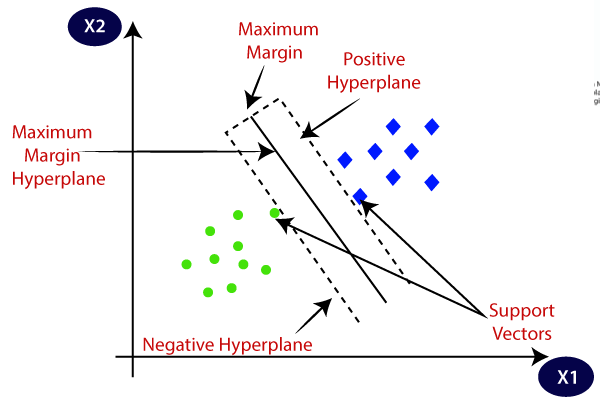
Concept: Support Vector Machines (SVMs) are a type of supervised learning algorithm that can be used for classification or regression problems. It finds the optimal boundary (hyperplane) that separates the classes with the maximum margin (distance) between the closest points of the classes (support vectors). These closest data points are called support vectors.

• Hyperplane: There can be multiple lines/decision boundaries to segregate the classes in n-dimensional space, but we need to find out the best decision boundary that helps to classify the data points. This best boundary is known as the hyperplane of SVM.
• Support Vectors: The data points or vectors that are the closest to the hyperplane and which affect the position of the hyperplane are termed as Support Vector. Since these vectors support the hyperplane, hence called a Support vector.

SVM can be of two types:

• Linear SVM: Linear SVM is used for linearly separable data, which means if a dataset can be classified into two classes by using a single straight line, then such data is termed as linearly separable data, and classifier is used called as Linear SVM classifier.
• Non-linear SVM: Non-Linear SVM is used for non-linearly separated data, which means if a dataset cannot be classified by using a straight line, then such data is termed as non-linear data and classifier used is called as Non-linear SVM classifier.

SVMs are particularly useful when the data is not linearly separable, which means that it cannot be separated by a straight line. In these cases, SVMs can transform the data into a higher dimensional space using a technique called kernel trick, where a non-linear boundary can be found. Some common kernel functions used in SVMs are polynomial, radial basis function (RBF), and sigmoid.

Mathematical Explanation:

• The goal is to maximize the margin, defined as 2 / ∣∣w∣∣ where w is the vector of coefficients for the features.
• The decision boundary is represented by w⋅x + b = 0, where b is the bias term.
• SVM tries to find www and bbb that maximize the margin while ensuring that the data points are classified correctly.

from sklearn.datasets import load_wine
from sklearn.svm import SVC
from sklearn.model_selection import train_test_split

# Load the wine dataset
X, y = load_wine(return_X_y=True)

# Split the data into training and testing sets
X_train, X_test, y_train, y_test = train_test_split(X, y, test_size=0.2, random_state=42)

# Create and train the model
model = SVC(kernel='linear', random_state=42)
model.fit(X_train, y_train)

# Make predictions
y_pred = model.predict(X_test)

print("Predictions:", y_pred)

5. Naive Bayes

Concept: Naive Bayes is a simple and efficient machine learning algorithm that is based on Bayes’ theorem and is used for classification tasks. It is called “naive” because it makes the assumption that all the features in the dataset are independent of each other, which is not always the case in real-world data.

The algorithm calculate the probability of a given class, given the values of the input features. Bayes’ theorem states that the probability of a hypothesis (in this case, the class) given some evidence (in this case, the feature values) is proportional to the probability of the evidence given the hypothesis, multiplied by the prior probability of the hypothesis.

Naive Bayes algorithm can be implemented using different types of probability distributions such as Gaussian, Multinomial, and Bernoulli. Gaussian Naive Bayes is used for continuous data, Multinomial Naive Bayes is used for discrete data, and Bernoulli Naive Bayes is used for binary data.

Mathematical Explanation:

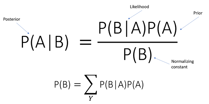
• P(A∣B) is the probability of event A given that B is true.
• P(B∣A) is the probability of event B given that A is true.
• P(A) and P(B) are the probabilities of A and B independently.

from sklearn.datasets import load_digits
from sklearn.naive_bayes import GaussianNB
from sklearn.model_selection import train_test_split

# Load the digits dataset
X, y = load_digits(return_X_y=True)

# Split the data into training and testing sets
X_train, X_test, y_train, y_test = train_test_split(X, y, test_size=0.2, random_state=42)

# Create and train the model
model = GaussianNB()
model.fit(X_train, y_train)

# Make predictions
y_pred = model.predict(X_test)

print("Predictions:", y_pred)

6. k-Nearest Neighbors (kNN)

Concept: K-Nearest Neighbors (KNN) is a simple and powerful algorithm for classification and regression tasks in machine learning. It is based on the idea that similar data points tend to have similar target values. The algorithm works by finding the k-nearest data points to a given input and using the majority class or average value of the nearest data points to make a prediction.

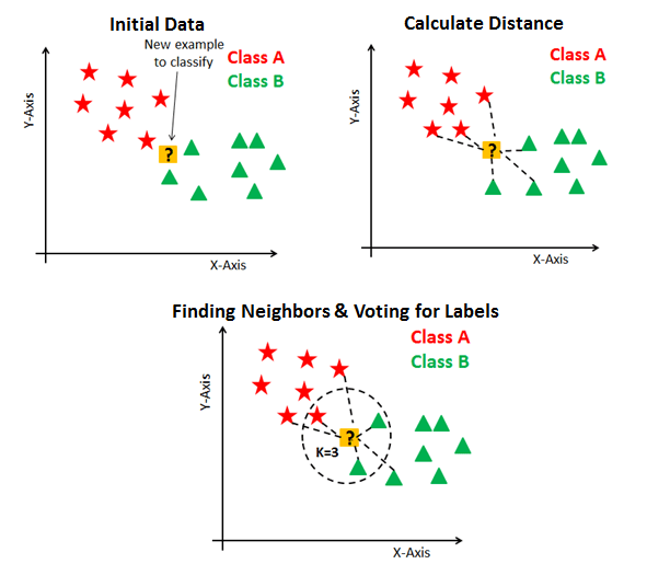
The process of building a KNN model begins with selecting a value for k, which is the number of nearest neighbors to consider for the prediction. The data is then split into training and test sets, with the training set used to find the nearest neighbors. To make a prediction for a new input, the algorithm calculates the distance (Euclidean) between the input and each data point in the training set, and selects the k-nearest data points. The majority class or average value of the nearest data points is then used as the prediction.

Mathematical Explanation:

One of the main advantages of KNN is its simplicity and flexibility. It can be used for both classification and regression tasks and does not make any assumptions about the underlying data distribution. Additionally, it can handle high-dimensional data and can be used for both supervised and unsupervised learning.

The main disadvantage of KNN is its computational complexity. As the size of the dataset increases, the time and memory required to find the nearest neighbors can become prohibitively large. Additionally, KNN can be sensitive to the choice of k, and finding the optimal value for k can be difficult.

from sklearn.datasets import load_iris
from sklearn.neighbors import KNeighborsClassifier
from sklearn.model_selection import train_test_split

# Load the iris dataset
X, y = load_iris(return_X_y=True)

# Split the data into training and testing sets
X_train, X_test, y_train, y_test = train_test_split(X, y, test_size=0.2, random_state=42)

# Create and train the model
model = KNeighborsClassifier(n_neighbors=3)
model.fit(X_train, y_train)

# Make predictions
y_pred = model.predict(X_test)

print("Predictions:", y_pred)

7. K-Means Clustering

Concept: K-means is an unsupervised machine-learning algorithm used for clustering. Clustering is the process of grouping similar data points together. K-means is a centroid-based algorithm, or distance-based algorithm, where we calculate the distances to assign a point to a cluster.

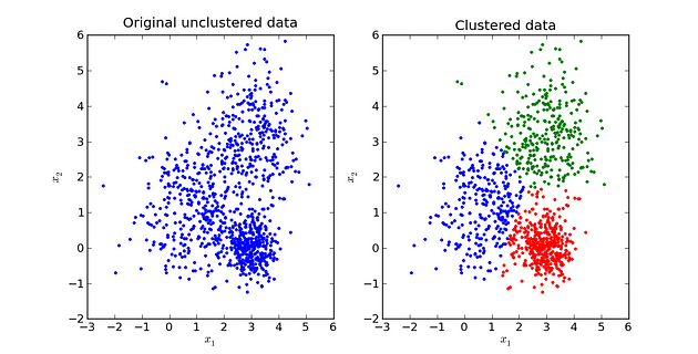
The algorithm works by randomly selecting k centroids, where k is the number of clusters we want to form. Each data point is then assigned to the cluster with the nearest centroid. Once all the points have been assigned, the centroids are recalculated as the mean of all the data points in the cluster. This process is repeated until the centroids no longer move or the assignment of points to clusters no longer changes.

Mathematical Explanation:

The algorithm works iteratively to minimize the within-cluster sum of squares (inertia):

• Initialize k centroids randomly.
• Assign each data point to the nearest centroid.
• Recalculate the centroids as the mean of all points in a cluster.
• Repeat steps 2 and 3 until the centroids do not change.

where μi is the centroid of cluster Ci.

One of the main advantages of KNN is its simplicity and flexibility. It can be used for both classification and regression tasks and does not make any assumptions about the underlying data distribution. Additionally, it can handle high-dimensional data and can be used for both supervised and unsupervised learning.

The main disadvantage of KNN is its computational complexity. As the size of the dataset increases, the time and memory required to find the nearest neighbors can become prohibitively large. Additionally, KNN can be sensitive to the choice of k, and finding the optimal value for k can be difficult.

from sklearn.datasets import make_blobs
from sklearn.cluster import KMeans

# Create a synthetic dataset
X, _ = make_blobs(n_samples=100, centers=3, n_features=2, random_state=42)

# Create and train the model
model = KMeans(n_clusters=3, random_state=42)
model.fit(X)

# Predict the clusters
labels = model.predict(X)

print("Cluster labels:", labels)

8. Random Forest

Concept: The idea behind using multiple decision trees is that while a single decision tree may be prone to overfitting, a collection of decision trees, or a forest, can reduce the risk of overfitting and improve the overall accuracy of the model.

The process of building a Random Forest begins with creating multiple decision trees using a technique called bootstrapping. Bootstrapping is a statistical method that involves randomly selecting data points from the original dataset with replacement. This creates multiple datasets, each with a different set of data points, which are then used to train individual decision trees.

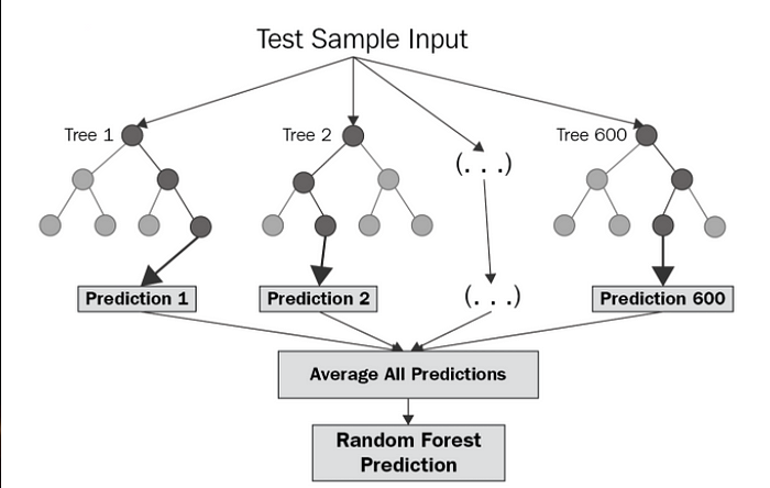
One of the main advantages of Random Forest is that it is less prone to overfitting than a single decision tree. The averaging of multiple trees smooths out the errors and reduces the variance. Random Forest also performs well in high-dimensional datasets and datasets with a large number of categorical variables.

The disadvantage of Random Forest is that it can be computationally expensive to train and make predictions. As the number of trees in the forest increases, the computational time increases as well. Additionally, Random Forest can be less interpretable than a single decision tree because it is harder to understand the contribution of each feature to the final prediction.

from sklearn.datasets import load_breast_cancer
from sklearn.ensemble import RandomForestClassifier
from sklearn.model_selection import train_test_split

# Load the breast cancer dataset
X, y = load_breast_cancer(return_X_y=True)

# Split the data into training and testing sets
X_train, X_test, y_train, y_test = train_test_split(X, y, test_size=0.2, random_state=42)

# Create and train the model
model = RandomForestClassifier(random_state=42)
model.fit(X_train, y_train)

# Make predictions
y_pred = model.predict(X_test)

print("Predictions:", y_pred)

9. Dimensionality Reduction Algorithms (PCA)

Concept: Dimensionality reduction is used to reduce the number of input variables in a dataset while retaining as much information as possible. It is used to improve the performance of machine learning algorithms and make data visualization easier. There are several dimensionality reduction algorithms available, including Principal Component Analysis (PCA), Linear Discriminant Analysis (LDA), and t-Distributed Stochastic Neighbor Embedding (t-SNE).

• Linear Discriminant Analysis (LDA) is a supervised dimensionality reduction technique that is used to find the most discriminative features for the classification task. LDA maximizes the separation between the classes in the lower-dimensional space.
• Principal Component Analysis (PCA) is a linear dimensionality reduction technique that uses orthogonal transformation to convert a set of correlated variables into a set of linearly uncorrelated variables called principal components. PCA is useful for identifying patterns in data and reducing the dimensionality of the data without losing important information.
• t-Distributed Stochastic Neighbor Embedding (t-SNE) is a non-linear dimensionality reduction technique that is particularly useful for visualizing high-dimensional data. It uses probability distributions over pairs of high-dimensional data points to find a low-dimensional representation that preserves the structure of the data.

One of the main advantages of dimensionality reduction techniques is that they can improve the performance of machine learning algorithms by reducing the computational cost and reducing the risk of overfitting. Additionally, they can make data visualization easier by reducing the number of dimensions to a more manageable number.

The main disadvantage of dimensionality reduction techniques is that they can lose important information in the process of reducing the dimensionality. Additionally, the choice of dimensionality reduction technique depends on the type of data and the task at hand, and it can be difficult to determine the optimal number of dimensions to retain.

from sklearn.datasets import load_digits
from sklearn.decomposition import PCA

# Load the digits dataset
X, y = load_digits(return_X_y=True)

# Apply PCA to reduce the number of features
pca = PCA(n_components=2)
X_reduced = pca.fit_transform(X)

print("Reduced feature set shape:", X_reduced.shape)

10. Gradient Boosting Algorithms

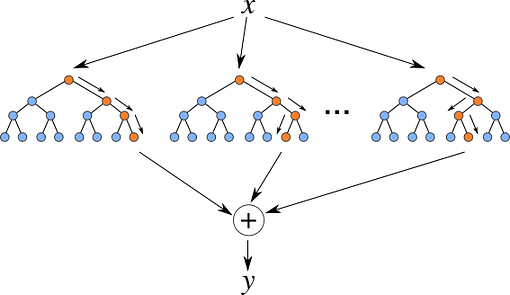
Concept: Gradient Boosting is an ensemble technique that builds models sequentially. Each new model corrects the errors made by the previous ones. This method is highly effective for both classification and regression tasks.

Mathematical Explanation:

• The model minimizes a loss function by adding models that predict the residuals (errors) of the previous models:

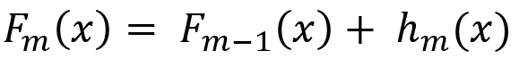
where:

• Fm(x) is the model after mmm iterations.
• hm(x) is the model that corrects the errors of Fm−1(x).

XGBoost, LightGBM, and CatBoost are popular implementations of Gradient Boosting.

import xgboost as xgb
from sklearn.datasets import load_breast_cancer
from sklearn.model_selection import train_test_split

# Load the breast cancer dataset
X, y = load_breast_cancer(return_X_y=True)

# Split the data into training and testing sets
X_train, X_test, y_train, y_test = train_test_split(X, y, test_size=0.2, random_state=42)

# Create and train the model
model = xgb.XGBClassifier(random_state=42)
model.fit(X_train, y_train)

# Make predictions
y_pred = model.predict(X_test)

print("Predictions:", y_pred)

Thanks for reading✨ If you like the article make sure to:

• 👏 Clap for the story (50 claps)
• For More content Visit DeepNexus 🚀 | Substack
• Follow me: LinkedIn | YouTube✅ | Github🐱