Time-Series Forecasting: Predicting Stock Prices Using An ARIMA Model

In this post I show you how to predict the TESLA stock price using a forecasting ARIMA model

1. Introduction

1.1. Time-series & forecasting models

Time-series forecasting models are the models that are capable to predict future values based on previously observed values. Time-series forecasting is widely used for non-stationary data. Non-stationary data are called the data whose statistical properties e.g. the mean and standard deviation are not constant over time but instead, these metrics vary over time.

These non-stationary input data (used as input to these models) are usually called time-series. Some examples of time-series include the temperature values over time, stock price over time, price of a house over time etc. So, the input is a signal (time-series) that is defined by observations taken sequentially in time.

A time series is a sequence of observations taken sequentially in time.

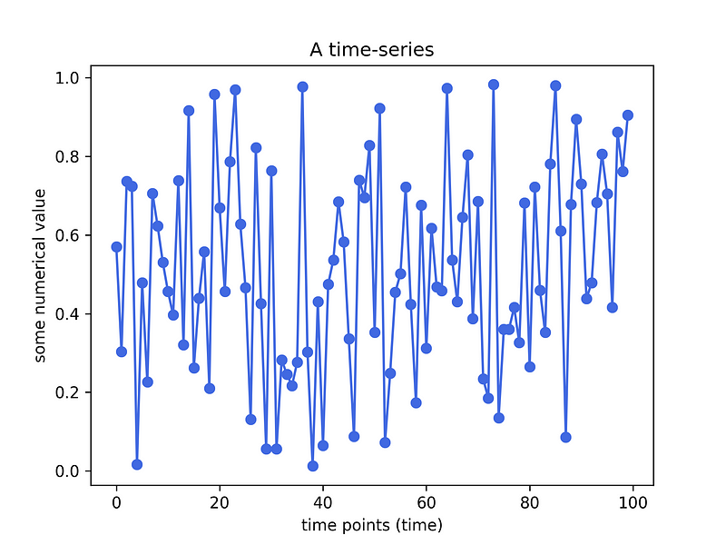
Observation: Time-series data is recorded on a discrete time scale.

Disclaimer: There have been attempts to predict stock prices using time series analysis algorithms, though they still cannot be used to place bets in the real market. This is just a tutorial article that does not intent in any way to “direct” people into buying stocks.

2. The AutoRegressive Integrated Moving Average (ARIMA) model

A famous and widely used forecasting method for time-series prediction is the AutoRegressive Integrated Moving Average (ARIMA) model. ARIMA models are capable of capturing a suite of different standard temporal structures in time-series data.

Terminology

Let’s break down these terms:

• AR: < Auto Regressive > means that the model uses the dependent relationship between an observation and some predefined number of lagged observations (also known as “time lag” or “lag”).
• I:< Integrated > means that the model employs differencing of raw observations (e.g. it subtracts an observation from an observation at the previous time step) in order to make the time-series stationary.MA:
• MA: < Moving Average > means that the model exploits the relationship between the residual error and the observations.

Model parameters

The standard ARIMA models expect as input parameters 3 arguments i.e. p,d,q.

• p is the number of lag observations.
• d is the degree of differencing.
• q is the size/width of the moving average window.

NEW: After a great deal of hard work and staying behind the scenes for quite a while, we’re excited to now offer our expertise through a platform, the “Data Science Hub” on Patreon (https://www.patreon.com/TheDataScienceHub). This hub is our way of providing you with bespoke consulting services and comprehensive responses to all your inquiries, ranging from Machine Learning to strategic data analytics planning.

3. Getting the stock price history data

Thanks to Yahoo finance we can get the data for free. Use the following link to get the stock price history of TESLA: https://finance.yahoo.com/quote/TSLA/history?period1=1436486400&period2=1594339200&interval=1d&filter=history&frequency=1d

You should see the following:

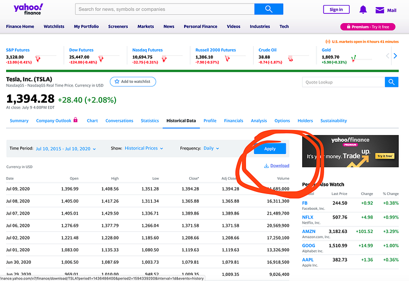
Click on the Download and save the .csv file locally on your computer.

The data are from 2015 till now (2020) !

4. Python working example

Modules needed: Numpy, Pandas, Statsmodels, Scikit-Learn

4.1. Load & inspect the data

Our imports:

import numpy as np 
import pandas as pd 
import matplotlib.pyplot as plt
from pandas.plotting import lag_plot
from pandas import datetime
from statsmodels.tsa.arima_model import ARIMA
from sklearn.metrics import mean_squared_error

Now let’s load the TESLA stock history data:

df = pd.read_csv("TSLA.csv")
df.head(5)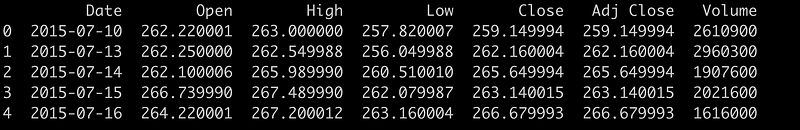

• Our target variable will be the Close value.

Before building the ARIMA model, let’s see if there is some cross-correlation in out data.

plt.figure()
lag_plot(df['Open'], lag=3)
plt.title('TESLA Stock - Autocorrelation plot with lag = 3')
plt.show()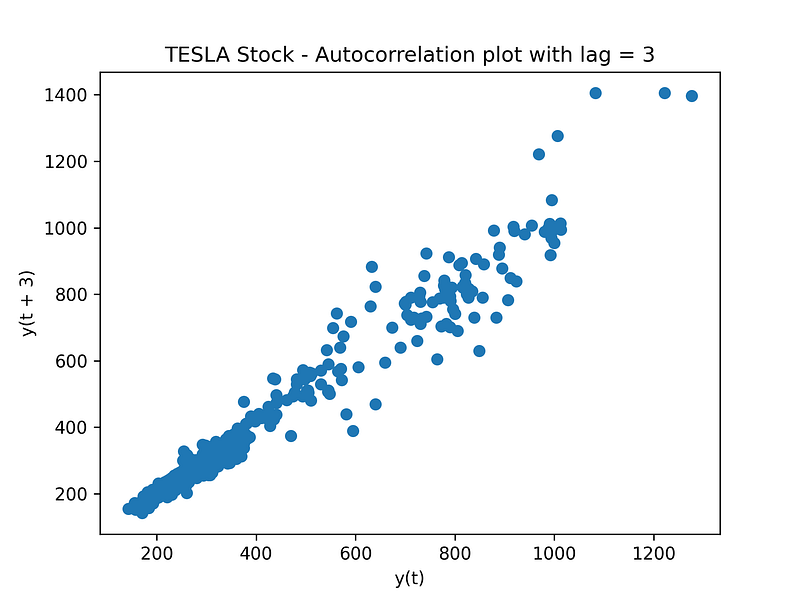

We can now confirm that ARIMA is going to be a good model to be applied to this type of data (there is auto-correlation in the data).

Finally, let’s plot the stock price evolution over time.

plt.plot(df["Date"], df["Close"])
plt.xticks(np.arange(0,1259, 200), df['Date'][0:1259:200])
plt.title("TESLA stock price over time")
plt.xlabel("time")
plt.ylabel("price")
plt.show()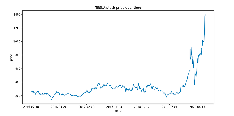

4.2. Build the predictive ARIMA model

Next, let’s divide the data into a training (70 % ) and test (30%) set. For this tutorial we select the following ARIMA parameters: p=4, d=1 and q=0.

train_data, test_data = df[0:int(len(df)*0.7)], df[int(len(df)*0.7):]

training_data = train_data['Close'].values
test_data = test_data['Close'].values

history = [x for x in training_data]
model_predictions = []
N_test_observations = len(test_data)

for time_point in range(N_test_observations):
    model = ARIMA(history, order=(4,1,0))
    model_fit = model.fit(disp=0)
    output = model_fit.forecast()
    yhat = output[0]
    model_predictions.append(yhat)
    true_test_value = test_data[time_point]
    history.append(true_test_value)

MSE_error = mean_squared_error(test_data, model_predictions)
print('Testing Mean Squared Error is {}'.format(MSE_error))

Summary of the code

• We split the training dataset into train and test sets and we use the train set to fit the model, and generate a prediction for each element on the test set.
• A rolling forecasting procedure is required given the dependence on observations in prior time steps for differencing and the AR model. To this end, we re-create the ARIMA model after each new observation is received.
• Finally, we manually keep track of all observations in a list called history that is seeded with the training data and to which new observations are appended at each iteration.

Testing Mean Squared Error is 741.0594879572484

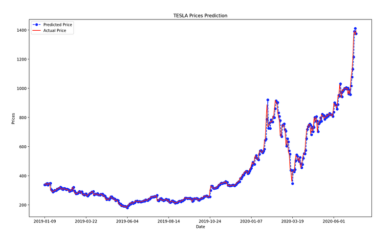
The MSE of the test set is quite large denoting that the precise prediction is a hard problem. However, this is the average squared value across all the test set predictions. Let’s visualize the predictions to understand the performance of the model more.

test_set_range = df[int(len(df)*0.7):].index

plt.plot(test_set_range, model_predictions, color='blue', marker='o', linestyle='dashed',label='Predicted Price')

plt.plot(test_set_range, test_data, color='red', label='Actual Price')

plt.title('TESLA Prices Prediction')
plt.xlabel('Date')
plt.ylabel('Prices')
plt.xticks(np.arange(881,1259,50), df.Date[881:1259:50])
plt.legend()
plt.show()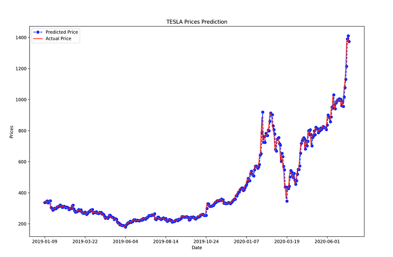

Not so bad right?

Our ARIMA model results in appreciable results. This model offers a good prediction accuracy and to be relatively fast compared to other alternatives, in terms of training/fitting time and complexity.

That’s all folks ! Hope you liked this article!

Stay tuned & support this effort

If you liked and found this article useful, follow me to be able to see all my new posts.

Questions? Post them as a comment and I will reply as soon as possible.

References

[1] https://en.wikipedia.org/wiki/Autoregressive_integrated_moving_average

Get in touch with me

• LinkedIn: https://www.linkedin.com/in/serafeim-loukas/
• ResearchGate: https://www.researchgate.net/profile/Serafeim_Loukas
• EPFL profile: https://people.epfl.ch/serafeim.loukas
• Stack Overflow: https://stackoverflow.com/users/5025009/seralouk