
Time series analysis using Prophet in Python — Part 1: Math explained
Check out the video version here:
Prophet models time series as a generalized additive model (GAM) combining the trend function, seasonality function, holiday effects, and an error term in one model:

- 𝑔(𝑡) : trend (non-periodic changes)
- 𝑠(𝑡): seasonality (periodic changes)
- ℎ(𝑡) : holiday effect
- 𝜖𝑡: error term, default prior 𝜖∼𝑁(0,0.5)
1. Trend model
Logistic trend model
The logistic trend model is based on the logistic growth model:
𝑔(𝑡)=𝐶/(1+exp(−𝑘(𝑡−𝑚))
C: carrying capacity
k: growth rate
m: offset parameter
Here is an example plotting g(t) with m=0 and t from 0 to 49. As we can see here, carrying capacity and growth rate may change and the resulting logistic growth model will look very differently.
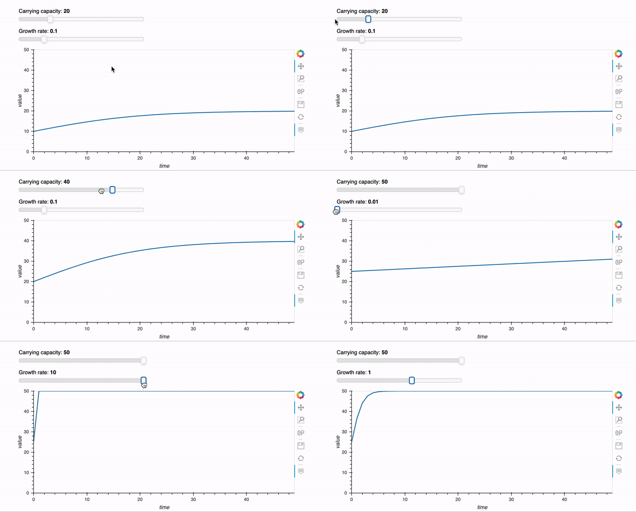
syntax for the plot:
Carrying capacity can change over time
To indicate that the carrying capacity is a function of time. We can write C as C(t).
Growth rate can change overtime
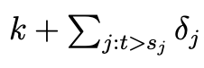
With 𝛿𝑗 change in growth rate at time 𝑠𝑗, growth rate becomes:
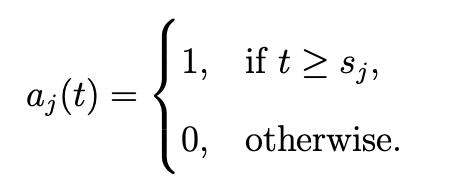
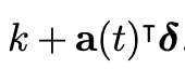
Here is another way to write this equation. We can vectorize the change 𝛅 and create a vector 𝐚(𝑡) to indicate when change happens.
Growth rate at time t becomes:
With those two changes, the logistic trend model can be written as:

And similarly, the linear trend model can be written as:

Note that 𝛾 here is to adjust the offset parameter to connect the endpoints of segments.
Parameters
- 𝑐(𝑡) user defined
- Prior 𝑚∼𝑁(0,5)
- 𝑠𝑗 automatically selected by the model
- Prior δ𝑗∼𝐿𝑎𝑝𝑙𝑎𝑐𝑒(0,𝜏)
- 𝜏 regularizes trend flexibility
- 𝛾 calculated based on other parameters
2. Seasonality model
Seasonality is modeled based on the Fourier series:

- N: order of Fourier series
- P: period
Which can be rewritten as 𝑋(𝑡)𝛽 with X(t) and 𝛽 specified as vectors:

Here is an example of the series and how the function changes regarding to a, b, N, and p (assuming a = a1 =… =aN and b = b1 =…= bN for simplicity).
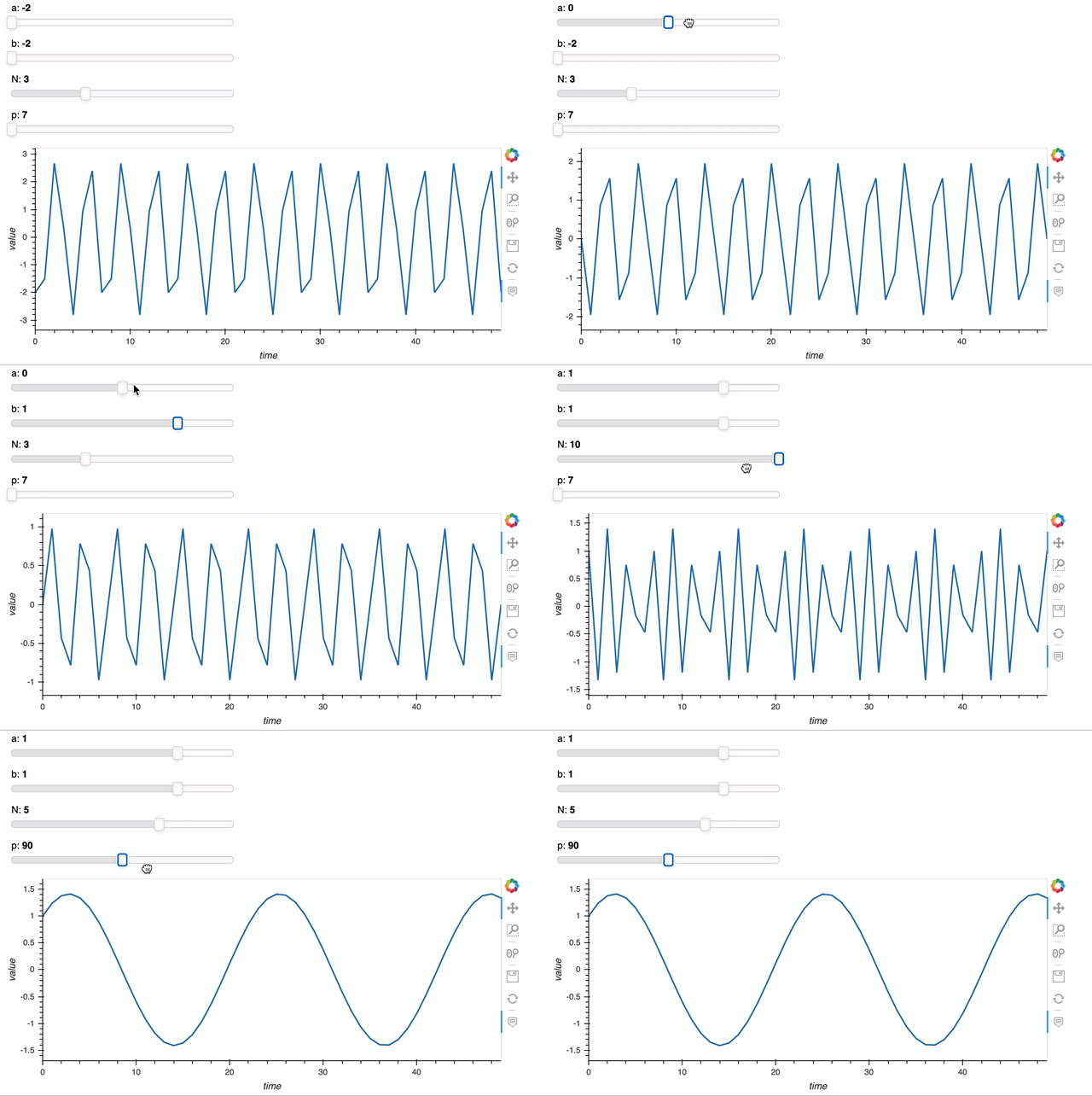
Syntax for this plot:
Parameters
- For yearly seasonality, default N=10, P=365.25
- For weekly seasonality, default N=3, P=7
- Prior 𝛽∼𝑁(0,𝜎^2). 𝜎 regularizes the strength of seasonality
3. Holiday model
Holiday model models the linear effect of the holidays, which is a vector of dummies (1 indicates holiday and 0 otherwise):
𝑍(𝑡)=[1(𝑡∈𝐷1),…,1(𝑡∈𝐷𝐿)]
ℎ(𝑡)=𝑍(𝑡)𝜅
Parameters
Prior 𝜅∼𝑁(0,𝜈^2)∼ default 𝑁(0,0.5)
Final model
Combining all three models together, we get the final model for our time series analysis:
𝑦|𝑚,𝛿,𝛽,𝜅,𝜖,∼𝑁(𝑔(𝑡)+𝑠(𝑡)+ℎ(𝑡),𝜖)
Then based on the priors of the parameters and the data, we can find maximum a posterior (MAP) estimates for all parameters.
What are the parameters we can tune in Prophet?
- growth
- Default: “linear”
- Alternative: “logistic
2. changepoint prior scale
- 𝜏τ
- Default: 0.05
- Higher value means more changepoints and more flexible trend
3. changepoint range:
- Defult: 0.8
- changepoints only apply to 80% of the data to better project forward and avoid overfitting at the end
4. seasonality prior scale
- 𝜎
- Default: 10
5. holidays_prior_scale
- 𝜈
- Default: 10
- Lower values means lower holiday effects. Reduce the value to avoid overfitting of the holiday effect.
6. seasonality_mode
- Default: “additive”, i.e., 𝑔(𝑡)+𝑠(𝑡)g(t)+s(t)
- Alternative : “multiplicative”, grows with the trend, i.e., 𝑔(𝑡)∗𝑠(𝑡)g(t)∗s(t)
7. yearly_seasonality
- Order of the Fourier series
- Default: False; if yearly_seasonality=True, default 10
- Higher value corresponds to higher frequent changes
8. weekly_seasonality
- Order of the Fourier series
- Default: 3
- Higher value corresponds to higher frequent changes
Other features:
- Locations of changepoints
- automatic detected
- can be specified using
changepoints = [dates]
2. Specify seasonalities
- Defaults: weekly and yearly seasonalities
- can add additional seasonalities (e.g., monthly) using
add_seasonality
3. Additional regressors
- we can add additional regressors using
add_regressor
4. Uncertainty
- Trend: we assume similar trend changes in the future. Higher changepoint prior scale lead to higher uncertainty.
- Seasonality: we need to use MCMC sampling to get the uncertainty in seasonality
Next, I am going to show you how to use Prophet and how to tune your model in practice. Check it out!
Ref:


