
Time Series Analysis & Forecasting
A Gentle Introduction to Time Series Analysis and Forecasting

Definition
A time series is a sequence of observations indexed by time. This means that the observations follows a particular order. The subscript t represents the set of allowed times T:
{xt} with t1 … tn Time series measures how something changes over time.
Applications of Time Series Analysis
There are three main application areas in time series analysis:
- Time series forecasting: The focus is to predict the future values of a time series.
- Time series classification: The goal is to predict an action based on past values.
- Causality: The aim is to drive inference from the relationships among related time series.
We’ll focus on time series forecasting. Some examples of problems where time series forecasting can help are:
- What is the expected sales volume of food groups in different stores in the next three months?
- What is the resale value of cars after leasing out for three years?
- What is the closing price of a stock each day?
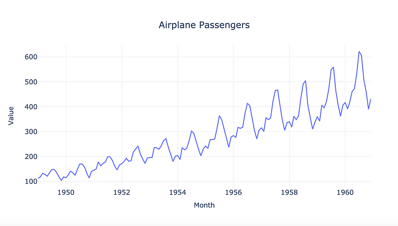
- What are passenger numbers for an international airline route?
Types of Time Series
We distinguish between two types of time series:
- Regular
- Irregular
The observations of regular time series have a regular interval of time. Those intervals could be every minute, every hour, or every month. This means that the time difference between each data point is the same. The observations of irregular time series don’t follow a regular interval of time. In the Airplane Passengers Dataset, the observations occur every month.
Components of Time Series
A time series consists of the following three components:
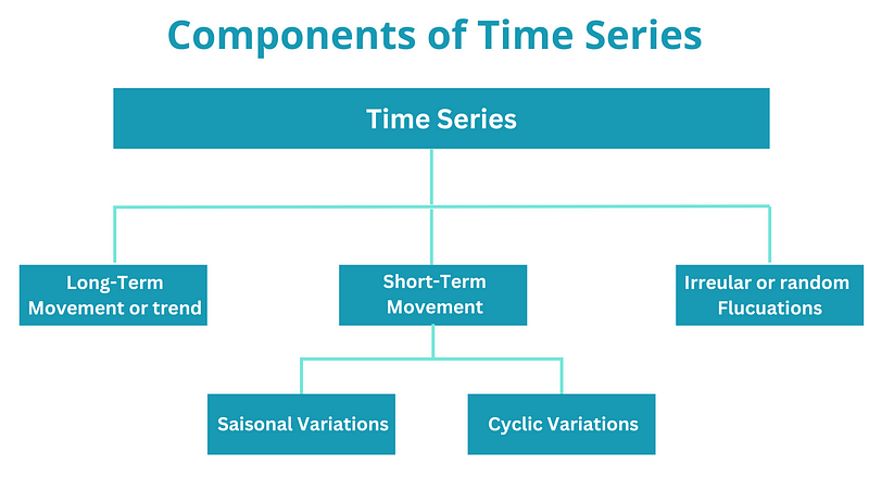
Long-term movement or trend
A trend is the long-term movement in which time series values are developing during a period. The change can be either:
- Upward (increase in level)
- Downward (decrease in level)
Short-term movements
There are two types of short-term movements:
- Seasonal movements are temporal fluctuations that usually occurs at a specific, regular intervals. Those movements are less than a year. It can occur on different time spans, such as daily, weekly, monthly, or yearly variation. Different social conventions, weather seasons, and climatic conditions are reasons for seasonal variations.
- Cyclic movements are recurrent patterns when data exhibits rises and falls.
Random or irregular fluctuations (Residual)
There is a variability that is irregular. These fluctuations are uncontrollable, unpredictable, and erratic. One examples are Bank holidays which can fall on different calendar days each year. Another examples are promotional campaigns which could depend on different business decisions.
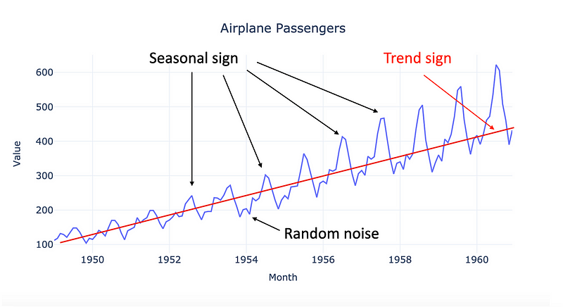
The first three components are also known as signals. The last component, random or irregular fluctuations, is also known as noise.
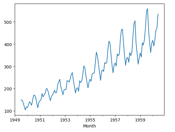
The Airplane Dataset shows a long-term linear (upward) trend with increasing, seasonal variations. But the seasonal fluctuations increase as the time series increases in size.
To remove the component effects, we will perform a decomposition process.
Decomposition a Time Series
In this section, we learn how to visualise time series into its components. The seasonal decomposition is the process of deconstructing a time series. The modeling of the decomposed components can be either additive or multiplicative.
Additive Model
We can reconstruct a time series by adding all three components:
Yt = Tt + St + RtWe’ll choose an additive model if the seasonal components do not change over time.
Multiplicative Model
We can also reconstruct a time series by multiplying all three components:
Yt = Tt * St * RtA multiplicative model is suitable when the seasonal variation fluctuates over time.
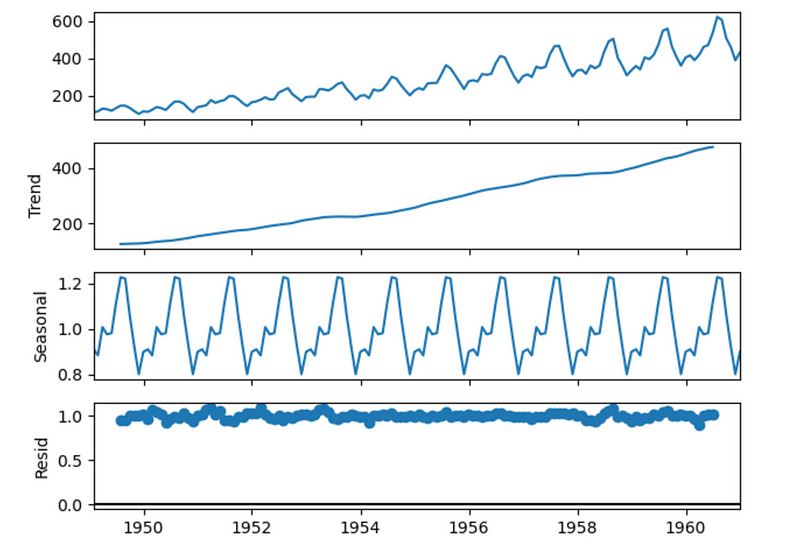
There are different implementations to decompose time series. We will use the seasonal_decompose function from the statsmodel library. It is an implementation that uses moving averages and period-adjusted averages. It supports both additive and multiplicative models of decomposition. Here, we should use the multiplicative model.
ts_decomposed = seasonal_decompose(ts,model=’multiplicative’)
ts_decomposed.plot()
pyplot.show()
The result looks as follow:
We can multiply the components to reconstruct the time series.
(ts_decomposed.trend * ts_decomposed.seasonal * ts_decomposed.resid).plot()
It gives the following plot as output.
Different Decomposition Techniques
In the next section, we’ll describe techniques to decompose time series. The general approach is as follows:
- Detrending: We estimate the trend component and remove it from the time series
- Deseasonalising: We estimate the seasonality component from the detrended time series.
- The remaining part of the time series is the residual.
Detrending
There are two different ways:
- Moving Average
- Locally estimated scatterplot smoothing (LOESS)
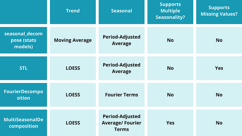
The moving average is a window moved along the time series in steps. LOESS is a non-parametric method used to fit a smooth curve onto a noisy signal. We will focus on the Moving Average.
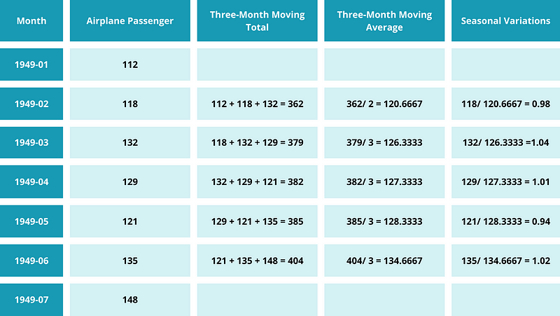
At each step, we’ll record the average of all the values in the window. This moving average helps us to estimate the slow change in time series or trend. We can also calculate the seasonal variations as difference between passengers and trend. The seasonal variations are not absolute values, because we use the multiplicative model. The disadvantage is that it is quite noisy. From our example, we can see a trend from February 1949 to August 1949.
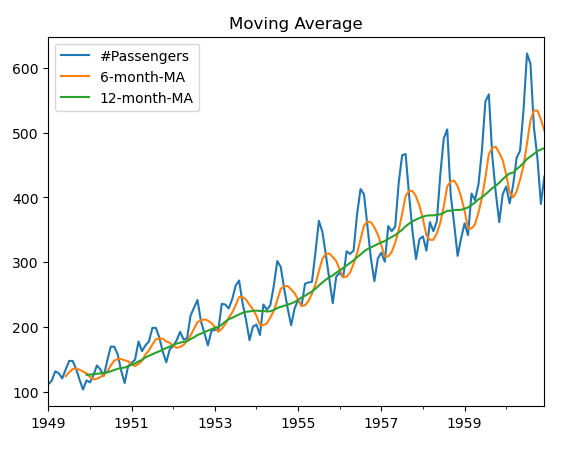
The Pandas DataFrame class offers a rolling function to calculate rolling windows. We will provide the seize of the moving window. We can either provide a fixed number of observations used for each window or a time delta. We will provide 6 months for the first window and 12 months for the second window.
ts['6-month-MA'] = ts['#Passengers'].rolling(window=6).mean()
ts['12-month-MA'] = ts['#Passengers'].rolling(window=12).mean()
After that, we will use Pandas DataFrame plot function to make a plot of the DataFrame.
Characteristics of Time Series
One important characteristic of a time series is stationarity.
Stationarity
The properties of a time series do not change its distribution over time. In other words, the mean and variance remain constant over time. If a time series is stationarity, it means it has no trend and no seasonal variability. Thus, stationary time series processes are easier to analyse and to model. The reasons is that their properties are not dependent on time and will be the same in the future.
Two forms of Stationarity:
- Strong stationarity: All the parameters of a time series do not change over time.
- Weak stationarity: The mean and the auto-covariance function do not change over time.
There are four questions to check whether a time series is stationary or not:
- Does the mean change over time? In other words, is there a trend in the time series?
- Does the variance change over time? In other words, is the time series heteroscedastic?
- Does the time series exhibit periodic changes in mean? Or in other words, is there seasonality in the time series?
- Does the time series have a unit root?
To check whether a time series has a unit root, we will use the Augmented Dickey-Fuller (ADF) test. The null hypothesis is that the AR coefficient in an AR model of the time series is equal to 1. This means that the time series is non-stationary. The alternate hypothesis is that the AR coefficient in the AR model is less than 1.
In Python, we can use the statsmodel library to check for unit roots.
adfuller(ts[‘#Passengers’])The result of the adfuller test is a tuple. This tuple contains the test-statistic, p-value, and critical values at different confidence levels. Here, we will use the p-value. As the p-value is an easy way to check whether we can reject the null hypothesis or not. If the p-value is less than 0.05, there is a 95 % probability that the series do not have a unit root. Then the time series would be stationary from a unit root perspective. In our case, the p-value is 0.9918802434376408. This means that the time series is non-stationary. In other words, the time series does not have a constant variance over time.
Conclusion
This was an introduction to time series analysis. The code is on GitHub. If you like this article, please clap. If you wish to read similar articles from me, please follow me to receive an email whenever I publish a new article.
References
Atwan, T. (2022) Time Series Analysis with Python Cookbook. 1st ed. Packt Publishing. Available at: https://www.perlego.com/book/3553599/time-series-analysis-with-python-cookbook-pdf (Accessed: 18 November 2023).
Auffarth, B. (2021): Machine Learning for Time-Series with Python. 1st ed. Packt Publishing. Available at: https://www.perlego.com/book/3040281/machine-learning-for-timeseries-with-python-forecast-predict-and-detect-anomalies-with-stateoftheart-machine-learning-methods-pdf (Accessed: 11 November 2023)
Joseph, M. (2022) Modern Time Series Forecasting with Python. 1st ed. Packt Publishing. Available at: https://www.perlego.com/book/3791670/modern-time-series-forecasting-with-python-explore-industryready-time-series-forecasting-using-modern-machine-learning-and-deep-learning-pdf (Accessed: 16 October 2023)
Lazzeri, F. (2020) Machine Learning for Time Series Forecasting with Python. 1st ed. Wiley. Available at: https://www.perlego.com/book/2050082/machine-learning-for-time-series-forecasting-with-python-pdf (Accessed: 12 November 2023).


