Three Very Useful Functions of Pandas to Summarize the Data

Pandas count, value_count, and crosstab functions in details

Pandas library is a very popular python library for data analysis. Pandas library has so many functions. This article will discuss three very useful and widely used functions for data summarizing. I am trying to explain it with examples so we can use them to their full potential.

The three functions I am talking about today are count, value_count, and crosstab.

The count function is the simplest. The value_count can do a bit more and the crosstab function does even more complicated work with simple commands.

The famous Titanic dataset is used for this demonstration. Please feel free to download the dataset and follow along from this link:

First import the necessary packages and the dataset:

import pandas as pd
import numpy as np
import matplotlib.pyplot as plt
import seaborn as sns

df = pd.read_csv("titanic_data.csv")
df.head()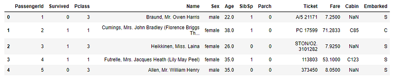

How many rows and columns are in the dataset?

df.shape

Output:

(891, 12)

The dataset has 891 rows of data and 12 columns.

Count

This is a simple function. But it is very useful for initial checking. We just learned that there are 891 rows in the dataset. In an ideal case, we should have 891 data in all 12 columns. But that doesn’t happen all the time. Most of the time we have to deal with null values. If you notice the first five rows of the dataset, there are some NaN values.

How much data are there in each column?

df.count(0)

Output:

PassengerId    891
Survived       891
Pclass         891
Name           891
Sex            891
Age            714
SibSp          891
Parch          891
Ticket         891
Fare           891
Cabin          204
Embarked       889
dtype: int64

In most columns, we have 891 data. But not in all the columns.

Let’s check the same for rows. How much real data are there in each row?

df.count(1)

Output:

0      11
1      12
2      11
3      12
4      11
       ..
886    11
887    12
888    10
889    12
890    11
Length: 891, dtype: int64

If there are indexes in the dataset, we can check the data count by index level. To demonstrate that I need to set indexes first. I will set two columns as indexes.

df = df.set_index(['Sex', 'Pclass'])
df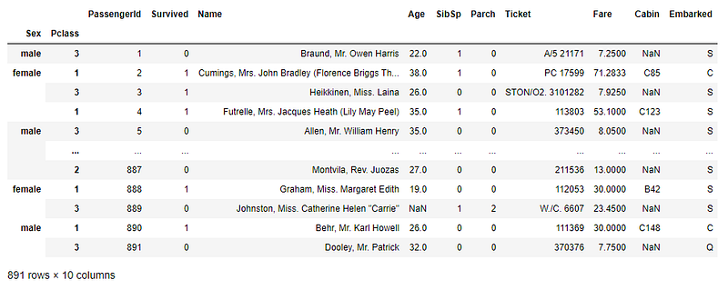

Now, the dataset has two indexes: ‘Sex’ and ‘Pclass’. Applying count on ‘Sex’ will show the data count of each gender:

df.count(level = "Sex")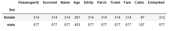

In the same way, applying count on ‘Pclass’ will show the data count of each passenger class of all the features:

df.count(level = 'Pclass')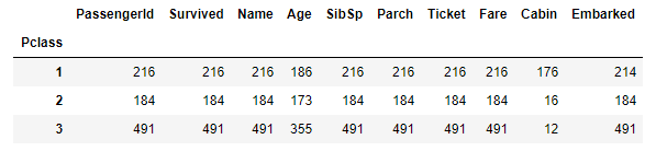

I just want to reset the index now to bring it back to its original shape:

df = df.reset_index()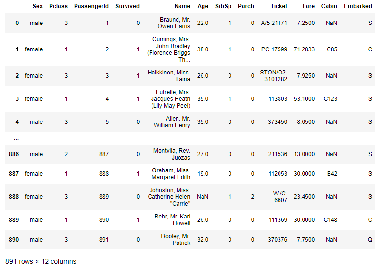

There is no index anymore.

Before, we saw how to get the data count for all the columns together. The next example shows how to get the data count for an individual column. Here is how to get the data count for the ‘Fare’ column for each ‘Pclass’.

df.groupby(by = 'Pclass')['Fare'].agg('count')

Output:

Pclass
1    216
2    184
3    491
Name: Fare, dtype: int64

You can also add a column with the data count of a single feature.

Here I am adding a new column name ‘freq’ that contains the data count of ‘Pclass’ for ‘Fare’.

df['freq'] = df.groupby(by='Pclass')['Fare'].transform('count')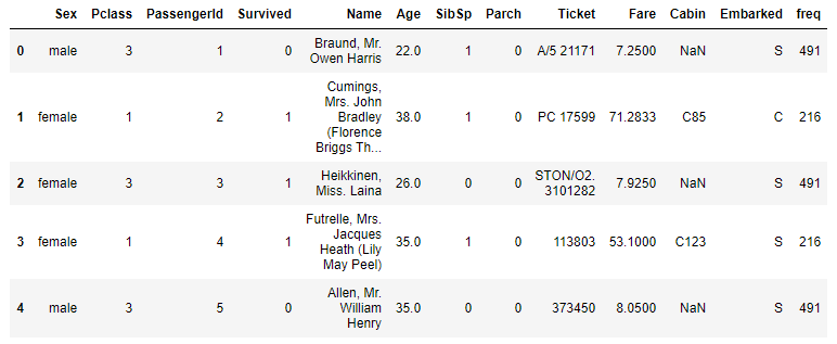

That was all for the count.

Value_Count

Value counts function is a bit more efficient in some respect. It is possible to achieve a bit more with a smaller amount of code. We used the group_by function and count to find the data count of individual ‘Pclass’ before. That can be done even more easily using value_count:

df['Pclass'].value_counts(sort = True, ascending  = True)

Output:

2    184
1    216
3    491
Name: Pclass, dtype: int64

Here not only we got the value count, but also got it sorted. If you do not need it sorted, just don’t use the ‘sort’ and ‘ascending’ parameters in it.

The values can be normalized as well using the normalize parameter:

df['Pclass'].value_counts(normalize=True)

Output:

3    0.551066
1    0.242424
2    0.206510
Name: Pclass, dtype: float64

One last thing I want to show on value_counts is the making of the bins. Here I divided the Fare into three bins:

df['Fare'].value_counts(bins = 3)

Output:

(-0.513, 170.776]     871
(170.776, 341.553]     17
(341.553, 512.329]      3
Name: Fare, dtype: int64

Crosstab

The crosstab function can do even more work for us in a single line of code. The most simple way of using crosstab is here:

pd.crosstab(df['Sex'], df['Pclass'])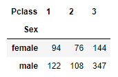

If it is necessary to get the total number at the end, we get the total for rows and columns both:

pd.crosstab(df['Sex'], df['Pclass'], margins = True, margins_name = "Total")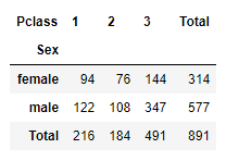

We can get the normalized values the way we did with the value counts function:

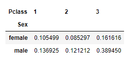
If you add all the values in this table that will be one. So, the normalization was done based on the total of all the values. But what if we need to normalize based on gender or Pclass only. That is also possible.

pd.crosstab(df['Sex'], df['Pclass'], normalize='columns')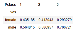

Each column adds up to 1. So, the table above shows the proportion of males and females of each ‘Pclass’.

We can normalize by the index of the table to find the proportion of people in ‘Pclass’ in each gender.

pd.crosstab(df['Sex'], df['Pclass'], normalize='index')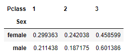

In the table above each adds up to 1.

The next example finds the mean ‘Fare’ for each ‘Pclass’ and each gender. The values are rounding up to 2 decimal points.

pd.crosstab(df['Sex'], df['Pclass'], values = df['Fare'], aggfunc = "mean").round(2)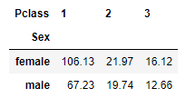

All this time we used one layer in the row direction and one layer in the column direction. Here, I am using two layers of data on the column direction:

pd.crosstab(df['Pclass'], [df['Sex'], df['Survived']])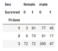

This table shows, how many people survived in each Passenger class per gender. Using the normalize function, we can find the proportion as well.

pd.crosstab(df['Pclass'], [df['Sex'], df['Survived']], normalize = 'columns')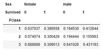

Let’s use two layers in the column and two layers in the rows:

pd.crosstab([df['Pclass'], df['Sex']], [df['Embarked'], df['Survived']],
           rownames = ['Pclass', 'gender'],
           colnames = ['Embarked', 'Survived'],
           dropna=False)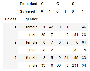

So much information packed in this one table. It looks even better and nicer in a heatmap.

import matplotlib.pyplot as plt
plt.figure(figsize=(8,6))

sns.heatmap(pd.crosstab([df['Pclass'], df['Sex']], [df['Embarked'], df['Survived']]), cmap = "YlGnBu",annot = True)
plt.show()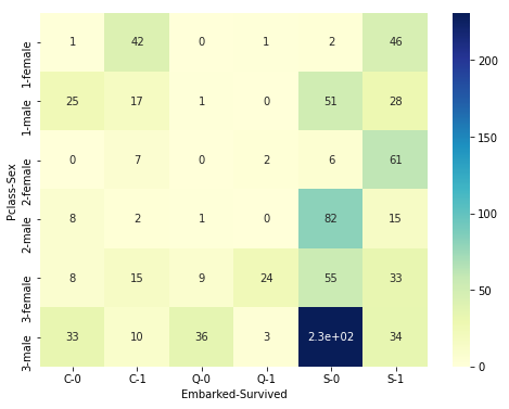

In the x-direction, it shows the ‘Embarked’ and ‘Survived’ data. In the y-direction, it shows the Passenger class and gender.

I have a video tutorial as well:

Conclusion

This article shows some very popular functions in detail to summarize the data. There are many ways to summarize the data. These are some simple and useful ways.

Feel free to follow me on Twitter and Facebook.

More Reading