This is how you can predict bitcoin future: Step by Step Guide

In this article i am going to show you, how you can forecast bitcoin price. We will use a simple LSTM model to do so. This is not the best attempt, but you will get your basic right.

#Installing yahoo finance
!pip install -q yfinance

This code quietly installs the yfinance package, enabling the user to use Yahoos financial data in the project without showing any installation messages. The installation runs silently in the background, and the user is notified only when its done. Its essential because the user needs yfinance to access Yahoo financial data.

#Importing Libraries
import pandas as pd
import numpy as np
from sklearn.preprocessing import MinMaxScaler
import matplotlib.pyplot as plt
import seaborn as sns
sns.set_style('whitegrid')
plt.style.use("fivethirtyeight")
%matplotlib inline

# For reading stock data from yahoo
from pandas_datareader.data import DataReader
import yfinance as yf

# For time stamps
from datetime import datetime

### Create the LSTM model
from tensorflow.keras.models import Sequential
from tensorflow.keras.layers import Dense
from tensorflow.keras.layers import LSTM

This script loads essential tools for analyzing stock data. It includes libraries like pandas, numpy, MinMaxScaler for data processing, and matplotlib and seaborn for plotting graphs. For fetching stock data from Yahoo, it uses pandas_datareader and yfinance. It also employs datetime to work with time-related data. The script prepares the notebook to show graphs directly in it by initializing matplotlib. It builds an LSTM a neural network good for time series analysis using components from tensorflow.keras.models and layers. Overall, the script prepares everything needed to start working on stock data with an LSTM neural network.

# Loading Data
# Defining the tickers or indices
tickers = ['BTC-USD', 'ETH-USD']

# Intializing the datetime as per today
end = datetime.now()
# Getting records of one year
start = datetime(end.year - 1, end.month, end.day)

# Extraction of stock data
df_btc= yf.download(tickers[0], start, end)
df_eth= yf.download(tickers[1], start, end)

The code starts by importing data, sets up BTC-USD and ETH-USD for tracking, and creates a current datetime object. It grabs the past years data by subtracting one year from todays date for the start date. Then it downloads the price information for Bitcoin and Ethereum using yf.download, saving it into df_btc and df_eth dataframes.

Closing Price

The closing price is the last price at which the stock is traded during the regular trading day. A stock’s closing price is the standard benchmark used by investors to track its performance over time.

# Bitcoin
df_btc.head()

# Exporting to csv
df_btc.to_csv('btc.csv')

This code loads Bitcoin data into a variable called df_btc, shows the first entries, and saves it as btc.csv. The .head function displays the initial data rows, while .to_csv saves the data to a file named btc.csv for later use or analysis.

# Summary Stats
df_btc.describe()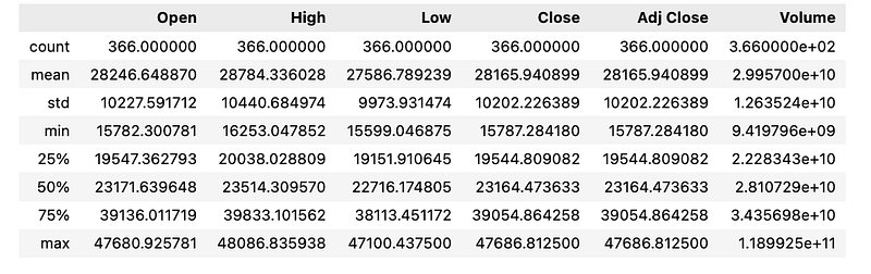

This code creates a simple summary of key stats like average, count, variation, and range for each column in the df_btc dataset, giving a quick overview of its data distribution.

# Plotting for adj closing price

fig, axes = plt.subplots(1,2,figsize=(15, 10))
df_btc['Close'].plot(ax=axes[0])
axes[0].set_title("BTC-USD")
axes[0].set_ylabel('Close')
df_eth['Close'].plot(ax=axes[1])
axes[1].set_title("ETH-USD")
axes[1].set_ylabel('Close')

    
plt.show()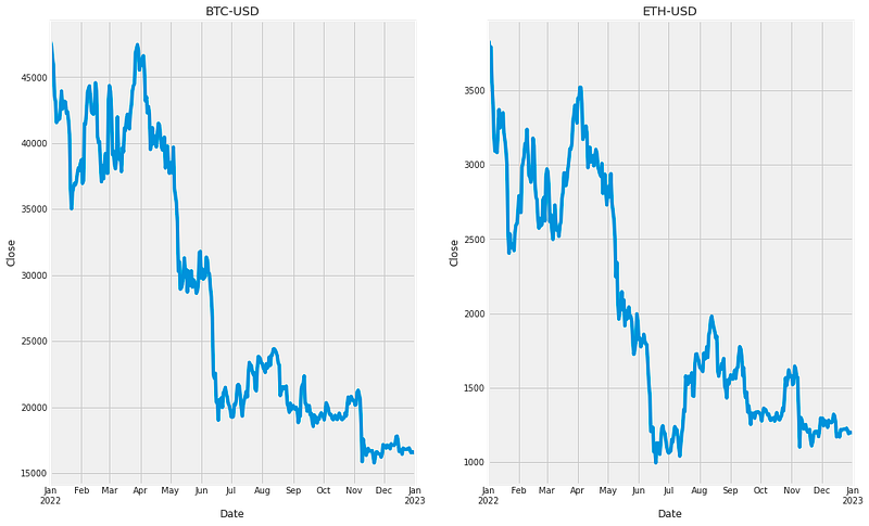

This code creates a chart to compare the adjusted closing prices of BTC and ETH. Using matplotlibs subplots, it makes a figure with two parts, one for each cryptocurrency, and sets the figure size. The BTC prices are plotted in the first part, with a title and y-axis label added. ETH prices are plotted in the second part, also with its title and label. The chart is then displayed with plt.show, making it simple to compare BTC and ETH prices.

# Using MinMaxScaler to scale the Close Attribute

scaler=MinMaxScaler(feature_range=(0,1))
btc=scaler.fit_transform(np.array(df_btc['Close']).reshape(-1,1))

The code uses the MinMaxScaler from sklearn to adjust the Close values in the df_btc DataFrame to a range between 0 and 1. The Close column is transformed into a numpy array with a new shape to match this scaling. This process normalizes the Close data, simplifying comparisons and analysis with other data in the set.

##splitting dataset into train and test split by 80% 
training_size=int(len(btc)*0.8)
test_size=len(btc)-training_size
train_data,test_data=btc[0:training_size,:],btc[training_size:len(btc),:1]

This code divides a dataset into training and testing parts. First, calculate the training set size as 80% of the datasets total rows. The rest will be for testing. Then, create train_data and test_data to store the respective data sets. Using slicing, select the first 80% of rows for train_data and the remaining rows for test_data, both for the first column, which has the bitcoin data. In short, the code splits the dataset for training and testing, selecting only the first column for both.

import numpy
# convert an array of values into a dataset matrix
def create_dataset(dataset, time_step=1):
 dataX, dataY = [], []
 for i in range(len(dataset)-time_step-1):
  a = dataset[i:(i+time_step), 0]   
  dataX.append(a)
  dataY.append(dataset[i + time_step, 0])
 return numpy.array(dataX), numpy.array(dataY)

The code has a function called create_dataset which turns a list of numbers into a matrix for analysis. It accepts the list and a time step value. As it loops through the list, it collects parts of the data into dataX and grabs the next value for dataY. In the end, it gives back these lists as numpy arrays. This process breaks down a big list into smaller chunks with a set number of steps, which is often done when working with data that changes over time in machine learning.

# reshape into X=t,t+1,t+2,t+3 and Y=t+4
time_step = 50
X_train, y_train = create_dataset(train_data, time_step)
X_test, ytest = create_dataset(test_data, time_step)

The first line of code arranges the data into groups of four consecutive numbers t, t+1, t+2, t+3, which will be fed into a neural network. Then, a function called create_dataset generates the train and test datasets, with a time step of 50. For the training dataset, it pairs the first 49 numbers as input X with the 50th number as the target output y, and keeps shifting one number forward to make more X, y pairs until it uses all the train data. It does the same for the test dataset. In the end, we have training and testing data made up of these input-output pairs, ready to train and test the network.

# reshape input to be [samples, time steps, features] which is required for LSTM
'''
LSTM needs 3D shape therefore it needs to be change
'''
X_train =X_train.reshape(X_train.shape[0],X_train.shape[1] , 1)
X_test = X_test.reshape(X_test.shape[0],X_test.shape[1] , 1)

The code sets up the data for an LSTM model by reshaping the training and testing data X_train and X_test into a 3D format. It keeps the original number of samples, sets the second dimension to the number of time steps, and makes the third dimension 1 for the feature count. After reshaping, the data is ready for training and testing the model.

# Build the LSTM model
model = Sequential()
model.add(LSTM(128, return_sequences=True, input_shape= (X_train.shape[1], 1)))
model.add(LSTM(64, return_sequences=False))
model.add(Dense(25))
model.add(Dense(1))

This code creates a neural network model with two types of layers: LSTM and Dense. First, it uses the Sequential function to start the model. The initial LSTM layer has 128 neurons and outputs the entire sequence for later layers to use; it expects input data of a certain shape. The next LSTM layer has 64 neurons but only outputs the final element in the sequence. After those, two Dense layers with 25 and 1 neurons perform operations to generate the final output. This model is designed for both training and making predictions with data.

# Compile the model
model.compile(optimizer='adam', loss='mean_squared_error')

# Train the model
model.fit(X_train, y_train,validation_data=(X_test,ytest),epochs=500,batch_size=20,verbose=1)

This code trains a model with the adam optimizer and mean_squared_error loss. It learns from training data X_train, y_train and checks its accuracy on testing data X_test, y_test. The training runs for 500 times epochs using groups of 20 samples batch_size and displays progress verbose=1.

### Lets Do the prediction and check performance metrics
train_predict=model.predict(X_train)
test_predict=model.predict(X_test)

This code uses a trained model to make predictions on both the training and test datasets. The line train_predict=model.predictX_train calculates predictions for the training data and stores them in train_predict. The line test_predict=model.predictX_test does the same for the test data, saving the results in test_predict. We can then check how well the model is doing by comparing these predictions to the real outcomes.

### Plotting 
# shift train predictions for plotting
look_back=50
trainPredictPlot = numpy.empty_like(btc)
trainPredictPlot[:, :] = np.nan
trainPredictPlot[look_back:len(train_predict)+look_back, :] = train_predict

# shift test predictions for plotting
testPredictPlot = numpy.empty_like(btc)
testPredictPlot[:, :] = numpy.nan
testPredictPlot[len(train_predict)+(look_back*2)+1:len(btc)-1, :] = test_predict


# plot baseline and predictions
plt.plot(scaler.inverse_transform(btc))
plt.plot(trainPredictPlot)
plt.plot(testPredictPlot)
plt.title('BTC-USD Model')
plt.xlabel('Days', fontsize=18)
plt.ylabel('Close Price USD ($)', fontsize=18)
plt.legend(['Train', 'Val', 'Predictions'], loc='upper right')
plt.show()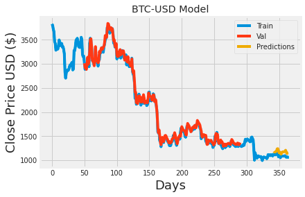

This code plots the models predictions for the Bitcoin to USD exchange rate. It begins by creating two empty arrays, trainPredictPlot and testPredictPlot, that match the size of the btc data array. These arrays are set up to hold the models predictions for training and testing data, respectively, and are offset to align with the actual Bitcoin data. The training predictions fill trainPredictPlot starting at index 50, while the testing predictions fill testPredictPlot from a further point, ensuring proper alignment. The code then displays a graph showing the Bitcoin data alongside the models predictions for both training and testing, making it easy to compare the predictions against actual exchange rates. The graph includes a title, axis labels, and a legend for clarity.

x_input=test_data[30:].reshape(1,-1)

temp_input=list(x_input)
temp_input=temp_input[0].tolist()
print(x_input)

This code processes the test_data starting from the 30th element, reshapes it into a 2D array with one row, and assigns it to a list named temp_input. It then flattens this list and prints out the 2D array. The purpose of the code is to prepare the data for further use or analysis.

# demonstrate prediction for next 30 days
from numpy import array

lst_output=[]
n_steps=44
i=0
while(i<30):
    
    if(len(temp_input)>44):
        #print(temp_input)
        x_input=np.array(temp_input[1:])
        print("{} day input {}".format(i,x_input))
        x_input=x_input.reshape(1,-1)
        x_input = x_input.reshape((1, n_steps, 1))
        #print(x_input)
        yhat = model.predict(x_input, verbose=0)
        print("{} day output {}".format(i,yhat))
        temp_input.extend(yhat[0].tolist())
        temp_input=temp_input[1:]
        #print(temp_input)
        lst_output.extend(yhat.tolist())
        i=i+1
    else:
        x_input = x_input.reshape((1, n_steps,1))
        yhat = model.predict(x_input, verbose=0)
        print(yhat[0])
        temp_input.extend(yhat[0].tolist())
        print(len(temp_input))
        lst_output.extend(yhat.tolist())
        i=i+1

print(lst_output)

This code uses the numpy library to work with arrays and performs the following steps: 1. Initializes an empty list named lst_output. 2. Sets the variable n_steps to 44 and starts a counter i at 0. 3. Enters a while loop that continues until the counter i hits 30. 4. Checks if the temp_input list has more than 44 items. If so, it takes 44 items from it to make the x_input. 5. Reshapes x_input into 1 row with n_steps columns. 6. Sends x_input to a machine learning model and gets a prediction of the next value. 7. Adds the predicted value to lst_output and prints it. 8. Appends the predicted value to temp_input and removes its first element. 9. Repeats these steps until i reaches 30. 10. If temp_input has 44 or fewer items, it reshapes x_input, predicts the next value, adds this to lst_output and temp_input, then increments i. 11. After the loop, it prints lst_output, which now has the predicted values for the next 30 days.

df3=btc.tolist()
df3.extend(lst_output)
plt.plot(df3[1200:])
df3=scaler.inverse_transform(df3).tolist()
btc_1=scaler.inverse_transform(btc).tolist()

#Demonstrating the forecast values using a plot
plt.title('BTC-USD Model')
plt.xlabel('Days', fontsize=18)
plt.ylabel('Close Price USD ($)', fontsize=18)
plt.plot(df3)
plt.plot(btc_1,color = "b")
plt.legend(['Current', 'Forecast'], loc='upper right')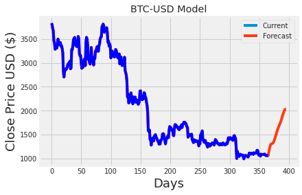

The code first turns the btc dataframe into a list and saves it as df3. It then adds another list, lst_output, to the end of df3. The merged list, which now contains data from btc and lst_output, is plotted using plt.plot starting from the 1200th index. The scaler.inverse_transform function is applied to df3 and the original btc dataframe to convert the scaled data back to its original values, with the transformed btc stored as btc_1. This step is needed because the data was scaled for the machine learning model. A graph named BTC-USD Model is then made, showing time on the x-axis and price on the y-axis, and it displays the data from both df3 and btc_1. A legend is added to differentiate between current and predicted values. In summary, the code integrates actual and forecasted data and provides a clear chart to show the results.