
The Values of Actions in Reinforcement Learning using Q-learning
The Q-learning algorithm implemented from scratch in Python

This article is a continuation of a series of articles about Reinforcement Learning (RL). Check out the other articles here:
All the codes used can be viewed here: https://github.com/Eligijus112/rl-snake-game
The notebook with all the plotting functions and agent training codes can be viewed here: https://github.com/Eligijus112/rl-snake-game/blob/master/chapter-6-qlearning.ipynb
In this article, I will present the reader with the concept of Q-values. For the sake of intuition, the reader can change the Q in Q-values for Quality-values. The q values are numeric values that assign a score for each action taken from each state:

The higher the score for a particular action in a given state, the better it is for the agent to take that action.
For example, if we can choose from state 1 to go either left or right, then if
Q(left, 1) = 3.187
Q(right, 1) = 6.588
Then the better action from state 1 which leads to more value is the “right” action.
An object that stores the q values is the q-table. The q-table is a matrix where each row is a state and each column is an action. We will denote such matrix as Q.
From the previous articles, let's remember some other important tables that are needed in Q-learning:
S — state matrix, which indexes all our states.
R — reward matrix, which indicates what rewards to we get for transitioning to a given state.
The value function V is not needed in Q learning, because we are not just interested in the value of a state but the value of a state-action pair.
Imagine that we have the following maze with 48 states:
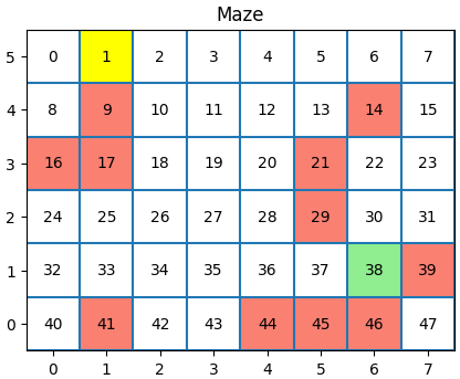
The yellow state is the state where our agent starts from (state 1).
The green state is the goal state (state 38).
The red states are the walls of the maze. If an agent chooses to go to the wall state, it is returned to the last state he was in with no reward. The same logic applies to going out of bounds.
The actions that our agent can take are represented by the vector [0, 1, 2, 3] which corresponds to [up, down, left, right].
The initial Q table for such an agent is the following:
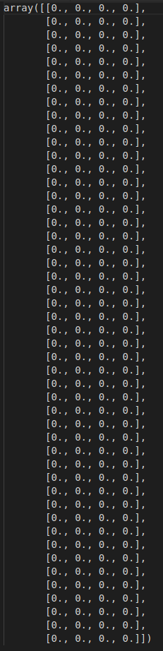
There are 48 rows indicating each state.
There are 4 columns representing the 4 actions our agent can take at each step: up, down, left or right.
The main objective of the Q-learning algorithm is to fill the above matrix so that our agent learns the most optimal path through the maze.
We will use a custom Agent class to implement the Q-learning algorithm:
class Agent:
    def __init__(
        self,
        nrow_maze: int,
        ncol_maze: int,
        actions: list = [0, 1, 2, 3],
        rewards: dict = {
            'step': 0.0,
            'wall': 0.0,
            'goal': 10,
        },
        gamma: float = 0.9,
        alpha: float = 0.1,
        epsilon: float = 0.1,
        seed: int = 42,
        ) -> None:
        """
        Creates an agent for the maze environment.

        Parameters
        ----------
        nrow_maze : int
            The number of rows in the maze.
        ncol_maze : int
            The number of columns in the maze.
        actions : list, optional
            A list of actions that the agent can take. The default is [0, 1, 2, 3].
            0: Up
            1: Down
            2: Left
            3: Right
        rewards : dict, optional
            A dictionary of rewards for the agent. The default is {'step': -1, 'wall': -10, 'goal': 10}.
        gamma : float, optional
            The discount factor. The default is 0.9.
        alpha : float, optional
            The learning rate. The default is 0.1.
        epsilon : float, optional
            The exploration rate. The default is 0.1.
        seed : int, optional
            The seed for the random generator. The default is 42.
        """
        self.nrow_maze = nrow_maze
        self.ncol_maze = ncol_maze
        self.rewards = rewards
        self.gamma = gamma
        self.alpha = alpha
        self.epsilon = epsilon
        self.seed = seed
        self.actions = actions

        # By default, the starting index is 0 0
        self.start_state = 0

        # By default, the goal index is the last index
        self.goal_state = nrow_maze * ncol_maze - 1

        # Creating the random generator with a fixed seed
        self.random_generator = np.random.default_rng(seed)

        # Creating the maze; We will denote it internaly as S
        self.init_S_table()

        # Initiating the Q-table
        self.init_Q_table()

        # Saving the initial past_action and past_state
        self.past_action = None
        self.past_state = None

        # Creating the action name dictionary
        self.action_name_dict = {
            0: 'up',
            1: 'down',
            2: 'left',
            3: 'right',
        }

        # Counter for the number of times our agent has seen the terminal state
        self.num_goal_reached = 0

        # Counter for each state and how many times the agent visited each
        self.state_visit_counter = {}

        # Empty dictionary of states visition paths
        self.state_visit_paths = {}

        # Placeholder for the current episode of learning
        self.current_episode = 0

  #####
  # OTHER METHODS BELLOW
  #####
The full Q-learning algorithm is as follows¹
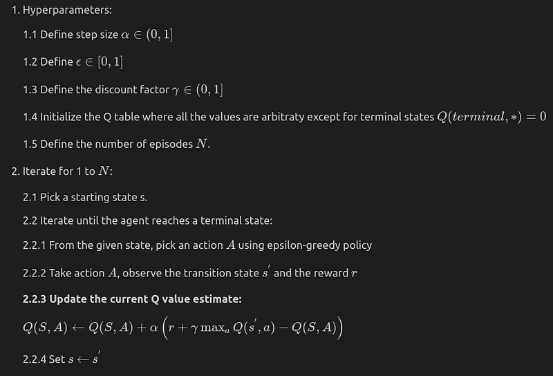
The epsilon-greedy strategy policy in step 2.2.1 is to take the action with the biggest Q value with the probability of 1 — epsilon and take a random action with the probability of epsilon.
The above policy is implemented in our agent by the following code:
def argmax(self, q_values: np.array):
        """argmax with random tie-breaking
        Args:
            q_values (Numpy array): the array of action values
        Returns:
            action (int): an action with the highest value
        """
        top = float("-inf")
        ties = []

        for i in range(len(q_values)):
            if q_values[i] > top:
                top = q_values[i]
                ties = []

            if q_values[i] == top:
                ties.append(i)

        return self.random_generator.choice(ties)

    def get_greedy_action(self, state: int) -> int:
        """
        Returns the greedy action given the current state
        """
        # Getting the q values for the current state
        q_values = self.Q[state]

        # Getting the greedy action
        greedy_action = self.argmax(q_values)

        # Returning the greedy action
        return greedy_action

    def get_epsilon_greedy_action(self, state: int) -> int:
        """
        Returns an epsilon greedy action
        """
        if self.random_generator.random() < self.epsilon:
            return self.get_action()
        else:
            return self.get_greedy_action(state)
The Q-learning step is the 2.2.3 step. In each state, our agent takes an action. Then, the learning is done by updating not only the current state the agent is in but the state-action pair Q(S, A). The most important part of the update rule is that we look at the state in which our agent ends up by taking action and then extracting the maximum value of that state from the Q table.
Let us examine the equation more closely:

The Q(S, A) is the state our agent is in and what action he has taken.
The
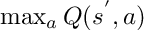
part is the maximum available Q value in the state where our agent ends up in, across all the actions.
The r is the reward of transitioning to a given state.
Everything else is user-defined hyperparameters.
Because we are using the algorithms' estimates for the updates of the Q-values, Q-learning falls under the bootstrapping methods family.
After every move that our agent takes, the Q table is updated.
The full implementation of the 2.2.3 step in our Agent class is the following:
def update_Q_table(self, new_state: int):
        """
        Function that applies the RL update function
        """
        # Getting the next_state's reward
        reward = self.reward_dict[new_state]

        # Saving the current Q value
        current_Q = self.Q[self.past_state][self.past_action]

        # If the new state is the terminal state or the wall state, then the max_Q is 0
        max_Q = 0

        # Else we get the max Q value for the new state
        if new_state != self.goal_state:
            new_state_Q_values = self.Q[new_state]

            # Getting the max Q value
            max_Q = np.max(new_state_Q_values)

        # Updating inplace the Q value
        self.Q[self.past_state][self.past_action] = current_Q + self.alpha * (reward + self.gamma * max_Q - current_Q)
The above function is called upon every move by our agent:
    def terminal_step(self, new_state: int):
        """
        Updates the agent one last time and resets the agent to the starting position
        """
        # Updating the Q table
        self.update_Q_table(new_state)

        # Resetting the agent
        self.past_state = self.start_state
        self.past_action = self.get_epsilon_greedy_action(self.past_state)

        # Incrementing the number of episodes
        self.current_episode += 1

    def get_next_state(self, s: int, action: int) -> int:
          """
          Given the current state and the current action, returns the next state index
          """
          # Getting the state coordinates
          s_row, s_col = self.get_state_coords(s)

          # Setting the boolean indicating that we have reached the terminal state
          reached_terminal = False

          # Getting the next state
          next_state = -1
          if action == 0:
              next_state = self.get_state_index(s_row - 1, s_col)
          elif action == 1:
              next_state = self.get_state_index(s_row + 1, s_col)
          elif action == 2:
              next_state = self.get_state_index(s_row, s_col - 1)
          elif action == 3:
              next_state = self.get_state_index(s_row, s_col + 1)

          # If next_state is a wall or the agent is out of bounds, we will stay in the same state
          if (next_state == -1) or (next_state in self.wall_states):
              return s, reached_terminal

          # If next_state is the goal state, we will return to the starting state
          if next_state == self.goal_state:
              # Incrementing the number of times our agent has reached the goal state
              self.num_goal_reached += 1
              reached_terminal = True

          # Returning the next state
          return next_state, reached_terminal

    def move_agent(self):
        """
        The function that moves the agent to the next state
        """
        # Getting the next state
        next_state, reached_terminal = self.get_next_state(self.past_state, self.past_action)

        # Updating the Q table
        if not reached_terminal:
            # Checking if the past_state is the same as the next_state; If that is true, it means our agent hit a wall
            # or went out of bounds
            if self.past_state != next_state:
                self.update_Q_table(next_state)

            # Setting the past_state as the next_state
            self.past_state = next_state

            # Getting the next action
            self.past_action = self.get_epsilon_greedy_action(self.past_state)
        else:
            self.terminal_step(next_state)
The above code snippet should be read from bottom to top.
At each movement, we check if are in a terminal state or not. If the agent steps in the terminal state, the Q-learning update equation simplifies to:

Lets us initiate our agent, train it for one episode and visualize the agent path:
  def train_episodes(self, num_episodes: int):
      """
      Function that trains the agent for one episode
      """
      # Calculating the episode number to end the training
      end_episode = self.current_episode + num_episodes - 1

      # Moving the agent until we reach the goal state
      while self.current_episode != end_episode:
          self.move_agent()
# Creating an agent object
agent = Agent(
nrow_maze=6,
ncol_maze=8,
seed=6,
rewards={'step': 0, 'goal': 10}
)
# Initiating the maze
agent.init_maze(maze_density=11)
# Training the agent for one episode
agent.train_episodes(num_episodes=1)
It took our agent 94 steps to reach the goal. At every step, the agent chooses an action in an epsilon-greedy way. In the first iteration, all the Q values are 0 for any transitioning state so the epsilon-greedy algorithm is the same as random wandering.
Let us inspect the Q table after one episode. The Q table is all zeroes except for the state 30:
agent.Q[30]

# Returns
# array([0., 1., 0., 0.])
The Q(30, 1) (meaning go “down” from state 30) has a value of 1. The equation by which this was calculated is:

Keep in mind that the initial Q(30, 1) = 0.
After one episode, we have only learnt one Q-value. Let us train one more episode:
# Training the agent for one episode
agent.train_episodes(num_episodes=1)

# Printing out the agent's 37 state
agent.Q[37]

# Returns
# array([0., 0., 0., 1.])
Now the agent wandered from the other side of the maze and learnt that going from state 37 to the right is the best choice.
What we would like to see is the number of steps that our agent makes to start decreasing as the episodes progress.
# Creating an agent object
agent = Agent(
    nrow_maze=6,
    ncol_maze=8,
    seed=6,
    rewards={'step': 0, 'goal': 10}
)

# Initiating the maze
agent.init_maze(maze_density=11)

# Letting the agent wonder for 1000 episodes
agent.train_episodes(100)
state_visits = agent.state_visit_paths
steps = [len(state_visits[episode]) for episode in state_visits]

# Ploting the number of steps per episode
plt.plot(steps)
plt.title("Number of steps per episode")
plt.xlabel("Episode")
plt.ylabel("Number of steps")
plt.show()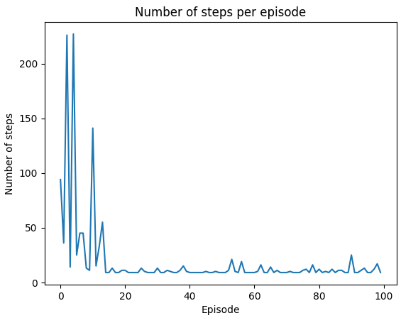
After the initial wandering, by episode 20 the agent has a stable policy to follow and takes around 10 steps to go from the starting position to the end position. The variation arises because we are still using the epsilon greedy algorithm to make a move and 10% of the time, a random action will be chosen.
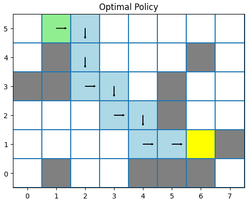
Now, the optimal greedy policy looks like this:
Additionally, our agent tracks how many times it was in any given state. We can plot that to see which states were the most popular during the training phase:
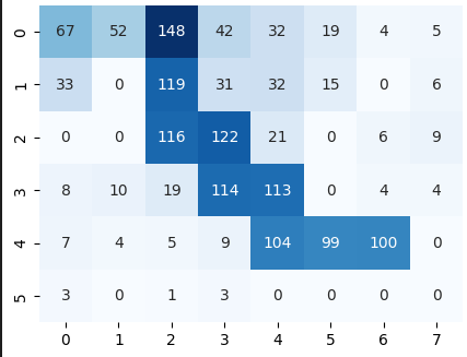
We can see that the agent quite often wandered to the left and the right from the starting state. But, because we let the agent take a random action only 10% of the time, the main path is the greedy one, meaning, the agent takes an action with the maximum Q value.
And lastly, we can plot the final agent traversal path:
To summarize:
- The Q-learning algorithm updates the values in the Q-table after every action the agent takes.
- Q-learning is a bootstrap algorithm because it uses its estimates to update the Q values.
- In Q-learning, we only need the state, reward and q tables for the full algorithm implementation.
- The main update rule in Q-learning is:
Happy coding and happy learning!
[1]
- Author: Richard S. Sutton, Andrew G. Barto
- Year: 2018
- Page: 131
- Title: Reinforcement Learning: An Introduction
- URL: http://archive.ics.uci.edu/ml


